Introduction
Overview
Teaching: 30 min
Exercises: 15 minQuestions
What is the basic syntax of the python programming language?
Objectives
Assign values to variables.
Use the print function to check how the code is working.
Use multiple assignment to assign several variables at once.
Link data to meaning using a dictionary
Getting Started
Python is a computer programming language that has become ubiquitous in scientific programming. Our initial lessons will run python interactively through a python interpreter. We will first use a Jupyter notebook. The [setup] page should have provided information on how to install and start a Jupyter notebook. Everything included in a code block is something you could type into your python interpreter and evaluate.
Setting up your Jupyter notebooks
In the [setup], you learned how to start a Jupyter notebook. Now, we will use the notebook to execute Python code. Jupyter notebooks are divided into cells. You run a Jupyter notebook one cell at a time. To execute a cell, click inside the cell and press shift+enter.
In the upper left corner, click where it says “Untitled” and change the name to “Introduction to Python”. We have now changed the name of the Jupyter Notebook.
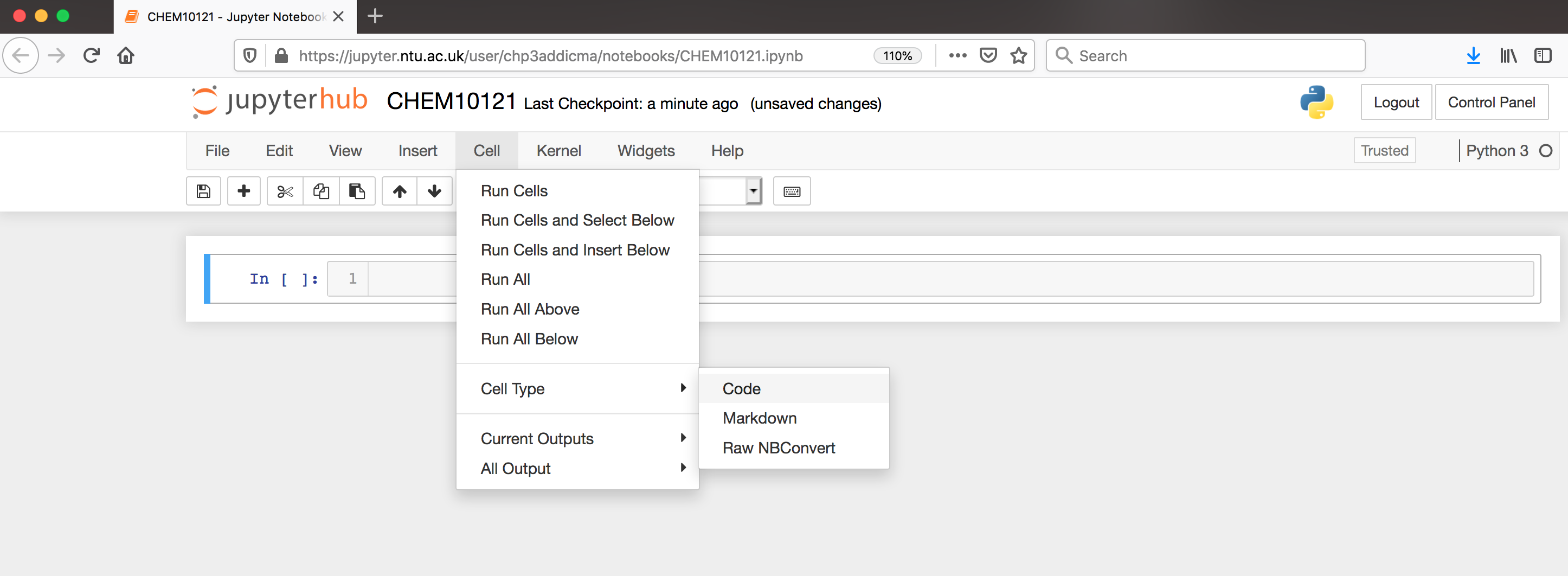
Jupyter notebooks allow us to also use something called markdown in some cells. We can use markdown to write descriptions about our notebooks for others to read. It’s a good practice to have your first cell be markdown to explain the purpose of the notebook. Let’s do that in our first cell. Click inside the first cell, then on the top of the screen select Cell->Cell Type->Markdown (shown below).
Now, return to the cell and type the following:
# Professional Development
## Introduction to Scientific Programming in Python

This lesson covers Python basics like variable creation and assignment and using the Jupyter notebook
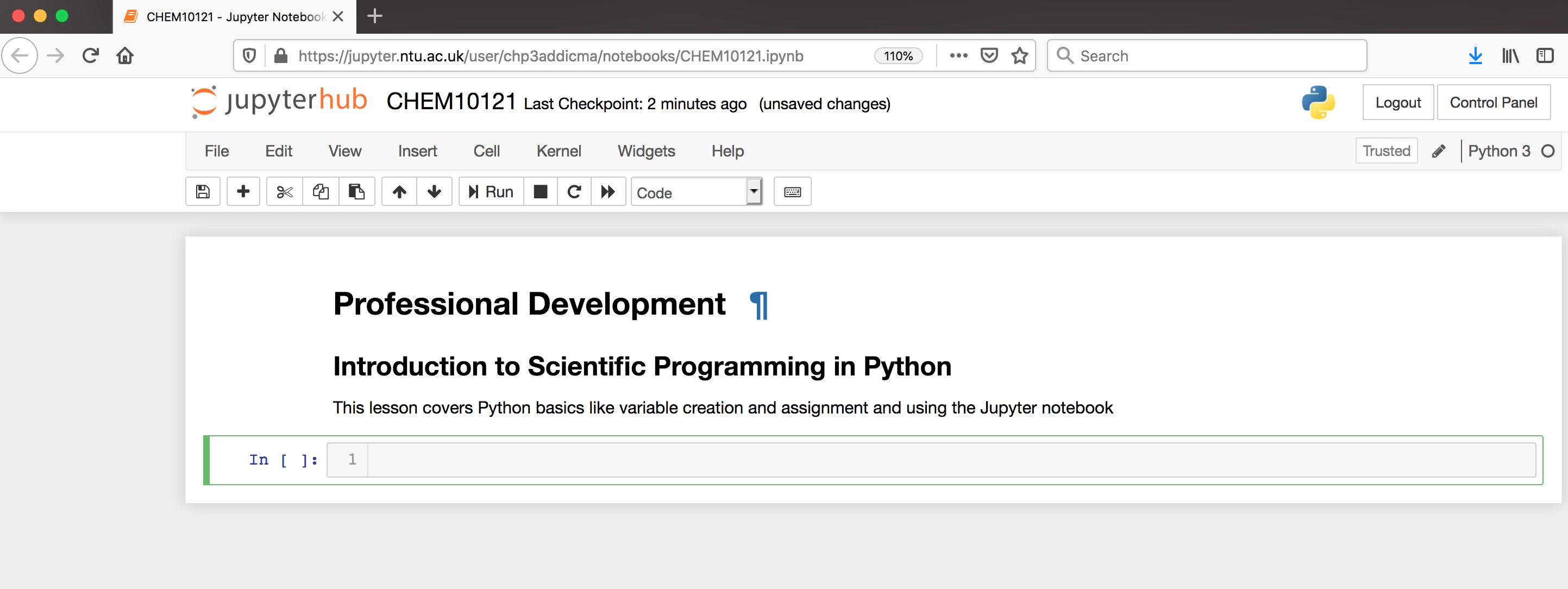
In Markdown, we create headers using a single # sign. Using two (##) creates a subheader. After typing this into a cell, press shift+enter to evaluate. Now your notebook should look like the following.
Now that our notebook is set-up, we’re ready to start learning some Python!
Saying Hello!
The very first thing we’ll do (because it’s obligatory) is get python to say Hello to us. Type the following into the next cell of your Jupyter notebook.
print("Hello World!")
Hello world!
Now let’s unpack what we did there:
Highlighted in green is the print() function. The print function tells python to print something to the screen. “Something” can be almost anything. The parentheses gather all the stuff that we’re sending to the print function. There are extra options we can use if we want to do something special (e.g. print to a file). A place with a whole pile of examples is here.
The final thing to note is that we used quotation marks to supply the string Hello World! as an argument to the print function. Why do you think we did that? What else could python think Hello World! was?
Variables
Let’s assign the string Hellow World! to a variable:
greeting = "Hello World!"
The syntax for assigning variables is the following:
variable_name = variable_value
Check your Understanding
What is printed by each of the following two statements?
print("greeting")
print(greeting)
Answer
greeting
Hello World!
- Variables can be strings, numbers, lots of other things
- Variable names can be (almost!) anything, but they should be readable. Think about reading your code later - “temperature_in_C” is informative, “t” is not.
- You can use any letter, any number and the underscore character
- In python, the name does not dictate the type of the data
Assigning variables and data types
Now let’s start working with some numbers. Any python interpreter can work just like a calculator. This is not very useful. Type the following into the next cell of your Jupyter notebook.
3 + 7
10
Here, Python has performed a calculation for us. To save this value, or other values, we assign it to a variable for later use.
Now let’s try a real calculation. Type the following into the next cell of your Jupyter notebook.
deltaH = -541.5   #kJ/mole
deltaS =  10.4     #kJ/(mole K)
temp = 298      #Kelvin
deltaG = deltaH - temp * deltaS
Notice several things about this code. The lines that begin with # are comment lines. The computer does not do anything with these comments. They have been used here to remind the user what units each of their values are in. Comments are also often used to explain what the code is doing or leave information for future people who might use the code.
We can now access any of the variables from other cells. Let’s print the value that we calculated. In the next cell,
print(deltaG)
-3640.7000000000003
At the beginning of this episode, we introduced the print() function. Often, we will use the print function just to make sure our code is working correctly.
Note that if you do not specify a new name for a variable, then it doesn’t automatically change the value of the variable; this is called being immutable. For example if we typed
print(deltaG)
deltaG * 1000
print(deltaG)
-3640.7000000000003
-3640.7000000000003
Nothing happened to the value of deltaG. If we wanted to change the value of deltaG we would have to re-save the variable using the same name to overwrite the existing value.
print(deltaG)
deltaG = deltaG * 1000
print(deltaG)
-3640.7000000000003
-3640700.0000000005
There are situations where it is reasonable to overwrite a variable with a new value, but you should always think carefully about this. Usually it is a better practice to give the variable a new name and leave the existing variable as is.
print(deltaG)
deltaG_joules = deltaG * 1000
print(deltaG)
print(deltaG_joules)
-3640700.0000000005
-3640700.0000000005
-3640700000.0000005
Assigning multiple variables at once
Python can do what is called multiple assignment where you assign several variables their values on one line of code. The following code block does the exact same thing as the previous code block.
#I can assign all these variables at once
deltaH, deltaS, temp = -541.5, 10.4, 298
deltaG = deltaH - temp * deltaS
print(deltaG)
-3640.7000000000003
Data types
Each variable is some particular type of data. The most common types of data are strings (str), integers (int), and floating point numbers (float). You can identify the data type of any variable with the function type(variable_name).
type(deltaG)
float
You can change the data type of a variable like this. This is called casting.
deltaG_string = str(deltaG)
type(deltaG_string)
str
Lists
Another common data structure in python is the list. Lists can be used to group several values or variables together, and are declared using square brackets [ ]. List values are separated by commas. Python has several built in functions which can be used on lists. The built-in function len can be used to determine the length of a list. This code block also demonstrates how to print multiple variables.
# This is a list
energy_kcal = [-13.4, -2.7, 5.4, 42.1]
# I can determine its length
energy_length = len(energy_kcal)

# print the list length
print('The length of this list is', energy_length)
The length of this list is 4
If you want to operate on a particular element of the list, you use the list name and then put in brackets which element of the list you want. In python counting starts at zero. So the first element of the list is list[0]
# Print the first element of the list
print(energy_kcal[0])
-13.4
You can use an element of a list as a variable in a calculation.
# Convert the second list element to kilojoules.
energy_kilojoules = energy_kcal[1] * 4.184
print(energy_kilojoules)
-11.296800000000001
Adding, subtracting and multiplying lists
Let’s test what we can do with lists. Start with two simple lists:
first_list = [3, 4, 7]
second_list = [2, 5, 1]
print(first_list + second_list)
[3, 4, 7, 2, 5, 1]
Adding lists together works the way we expect.
print(first_list - second_list)
---------------------------------------------------------------------------
TypeError                                 Traceback (most recent call last)
<ipython-input-28-2766c15298c3> in <module>
      1 first_list = [3, 4, 7]
      2 second_list = [2, 5, 1]
----> 3 print(first_list - second_list)

TypeError: unsupported operand type(s) for -: 'list' and 'list'
But subtracting lists does not.
print(first_list * second_list)
---------------------------------------------------------------------------
TypeError                                 Traceback (most recent call last)
<ipython-input-29-b239fdefe9ad> in <module>
      1 first_list = [3, 4, 7]
      2 second_list = [2, 5, 1]
----> 3 print(first_list * second_list)

TypeError: can't multiply sequence by non-int of type 'list'
We can’t multiply two lists either.
my_number = 3
print(first_list * my_number)
[3, 4, 7, 3, 4, 7, 3, 4, 7]
But we can multiply a list by an integer.
pop() and append()
Python has two other important functions that act on lists, pop() and append(). Try them out to learn what they do. Print the list and the value each time:
Try it out
print(first_list)
my_value = first_list.pop()
print('my_value is:', my_value)
print('The list is now', first_list)
print('The length of this list is', len(first_list))
first_list.append(8)
print('The list is now', first_list)
print('The length of this list is', len(first_list))
Answer
[3, 4, 7]
My_value is: 7
The list is now [3, 4]
The length of this list is 2
The list is now [3, 4, 8]
The length of this list is 3
Slices
Sometimes you will want to make a new list that is a subset of an existing list. For example, we might want to make a new list that is just the first few elements of our previous list. This is called a slice. The general syntax is
new_list = list_name[start:end]
When taking a slice, it is very important to remember how counting works in python. Remember that counting starts at zero so the first element of a list is list_name[0]. When you specify the last element for the slice, it goes up to but not including that element of the list. So a slice like
short_list = energy_kcal[0:2]
includes energy_kcal[0] and energy_kcal[1] but not energy_kcal[2].
print(short_list)
[-13.4, -2.7]
If you do not include a start index, the slice automatically starts at list_name[0]. If you do not include an end index, the slice automatically goes to the end of the list.
Check your Understanding
What does the following code print?
slice1 = energy_kcal[1:]
slice2 = energy_kcal[:3]
print('slice1 is', slice1)
print('slice2 is', slice2)
Answer
slice1 is [-2.7, 5.4, 42.1]
slice2 is [-13.4, -2.7, 5.4]
If you don’t specify a new variable name nothing happens. Looking at our example above if we only type
print(energy_kcal)
energy_kcal[0:2]
print(energy_kcal)
nothing happens to energy_kcal.
[-13.4, -2.7, 5.4, 42.1]
[-13.4, -2.7, 5.4, 42.1]
Dictionaries
Lists are great for keeping, well, lists. Let’s say you had a shopping list:
- flour
- eggs
- milk
- chocolate
- butter
But what if you have a recipe:
| Ingredient | Amount |
|---|---|
| flour | 2 |
| eggs | 2 |
| milk | 1 |
| chocolate | 0.75 |
| butter | 0.5 |
The amount of each ingredient is associated with the ingredient. Dictionaries are a way that python provides to keep variables together with their meanings. Because each value is associated with a key, some other languages call this construct an associative array.
Dictionaries are declared using braces { }. Key and value pairs are separated by commas. Like lists, python has several built in functions which can be used on dictionaries. The built-in function len can be used to determine the length of a dictionary. Dictionaries don’t have an order, you access the values by their key:
famous_chemists = {
"given_name": "Bettye",
"family_name": "Washington Greene",
"vintage": 1935
}
print(famous_chemists)
{'given_name': 'Bettye', 'family_name': 'Washington Greene', 'vintage': 1935}
We can add to a dictionary:
famous_chemists["university"] = "Wayne State University"
print(famous_chemists)
{'given_name': 'Bettye', 'family_name': 'Washington Greene', 'vintage': 1935, 'university': 'Wayne State University'}
Let’s check the length of the dictionary:
print(len(famous_chemists))
4
Now, this dictionary actually only describes a single chemist. A collection of famous chemists might be represented in python as a list of dictionaries or a dictionary of dictionaries
How to describe an atom?
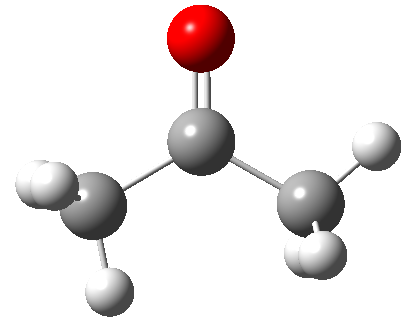
Below is depicted the acetone molecule. Think about how you would describe one of the carbon atoms using a python dictionary:
Design an atom homework
Design a dictionary that you could use to describe an atom. Think about the how to distinguish between the three carbon atoms in acetone and write a dictionary for each of the three carbon atoms. For now, make up any values you can’t guess.
atom = {
}
Hints
Consider how the left hand side carbon will differ from the central carbon.
What do you need to differentiate between the left hand side carbon and the one on the right?
A note about jupyter notebooks
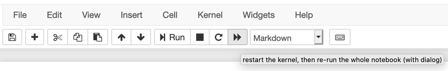
If you use the jupyter notebook for your python interpreter, the notebook only executes the current code block. This can have several unintended consequences. If you change a value and then go back and run an earlier code block, it will use the new value, not the first defined value, which may give you incorrect analysis. Similarly, if you open your jupyter notebook later, and try to run a code block in the middle, it may tell you that your variables are undefined, even though you can clearly see them defined in earlier code blocks. But if you didn’t re-run those code blocks, then python doesn’t know they exist. The same thing will occur if you save and close your notebook then reopen it. To rerun everything you’ve entered into a notebook, use the “fast forward” button at the top of the screen.
Key Points
You can assign the values of several variables at once.
Multiple values can be stored togeother in a list, which is ordered, or a dictionary, which is not ordered.
File Parsing
Overview
Teaching: 20 min
Exercises: 25 minQuestions
How do I sort through all the information in a text file and extract particular pieces of information?
Objectives
Use a for loop to perform the same action on the items in a list.
Use the append function to create new lists in for loops.
Open a file and read in its contents line by line.
Search for a particular string in a file.
Manipulate strings and change data types.
Print to a new file.
Repeating an operation many times: for loops
Often, you will want to do something to every element of a list. The structure
to do this is called a for loop. The general structure of a for loop is
for variable in list:
    do things using variable # This line is not executable python!
There are two very important pieces of syntax for the for loop. Notice the colon : after the word list. You will always have a colon at the end of a for statement. If you forget the colon, you will get an error when you try to run your code.
The second thing to notice is that the lines of code under the for loop (the things you want to do several times) are indented. Indentation is very important in python. There is nothing like an end or exit statement that tells you that you are finished with the loop. The indentation shows you what statements are in the loop. Each indentation is 4 spaces by convention in Python 3. However, if you are using an editor which understands Python, it will do the correct indentation for you when you press the tab key on your keyboard. In fact, the Jupyter notebook will notice that you used a colon (:) in the previous line, and will indent for you (so you will not need to press tab).
In the last episode, we had a list of energies in kcal. Let’s use a loop to change all of our energies in kcal to kJ.
for number in energy_kcal:
    kJ = number * 4.184
    print(kJ)
-56.0656
-11.296800000000001
22.593600000000002
176.1464
Now it seems like we are really getting somewhere with our program! But it would be even better if instead of just printing the values, it saved them in a new list. To do this, we are going to use the append function that we discovered in the last episode. The append function adds a new item to the end of an existing list. The general form of the append function is
list_name.append(new_thing) # This line would only work if you already had a list called `list_name` and a variable called `new_thing`
Try running this block of code. See if you can figure out why it doesn’t work.
for number in energy_kcal:
    kJ = number * 4.184
    energy_kJ.append(kJ)

print(energy_kJ)
---------------------------------------------------------------------------
NameError                                 Traceback (most recent call last)
<ipython-input-12-595146886489> in <module>()
      2 for number in energy_kcal:
      3     kJ = number*4.184
----> 4     energy_kJ.append(kJ)
      5
      6 print(energy_kJ)

NameError: name 'energy_kJ' is not defined
This code doesn’t work because on the first iteration of our loop, the list energy_kJ doesn’t exist. To make it work, we have to start the list outside of the loop. The list can be blank when we start it, but we have to start it.
energy_kJ = []
for number in energy_kcal:
    kJ = number * 4.184
    energy_kJ.append(kJ)

print(energy_kJ)
[-56.0656, -12.1336, 22.593600000000002, 176.1464]
Making choices: logic Statements
Within your code, you may need to evaluate a variable and then do something if the variable has a particular value. This type of logic is handled by an if statement. In the following example, we only append the negative numbers to a new list.
negative_energy_kJ = []

for number in energy_kJ:
    if number < 0:
        negative_energy_kJ.append(number)

print(negative_energy_kJ)
[-56.0656, -11.296800000000001]
Other logic operations include
- equal to
== - not equal to
!= - greater than
> - less than
< - greater than or equal to
>= - less than or equal to
<=
Notice that we use two equals signs (==) to check if two things are equal. Why?
If you are comparing strings, not numbers, you use different logic operators like is, in, or is not. We will see these types of logic operators used in our next lesson.
Compound comparisons
More than one condition can be checked at the same time, by using and, or, and not.
negative_numbers = []
for number in energy_kJ:
    if number < 0 or number == 0:
        negative_numbers.append(number)

print(negative_numbers)
[-56.0656, -11.296800000000001]
When using or for compound comparisons:
oris True if at least one condition is Trueoris False if all conditions are False
Sometimes you may want to check several conditions in sequence:
data_list_2 = [-12.23, 0, 0, 48.16, 48.21, 48.94, 0, 47.59]
correct_data = []
for number in data_list_2:
    if number < 0:
        print('data point is negative, discarding!')
    elif number == 0:
        print('data point is missing or zero!')
    else:
        correct_data.append(number)
data_average = sum(correct_data) / len(correct_data)
print("The number of data points is", len(correct_data))
print("The average of the points is", data_average)
data point is negative, discarding!
data point is missing or zero!
data point is missing or zero!
data point is missing or zero!
The number of data points is 4
The average of the points is 48.225
Exercise
The following list contains some floating point numbers and some numbers which have been saved as strings. Copy this list exactly into your code.
data_list = ['-12.5', 14.4, 8.1, '42']Set up a
forloop to go over each element ofdata_list. If the element is a string (str), recast it as a float. Save all of the numbers to a new list callednumber_list. Pay close attention to your indentation!Solution
data_list = ['-12.5', 14.4, 8.1, '42']
number_list = []
for item in data_list:
    if type(item) is str:
        item = float(item)
    number_list.append(item)

print(number_list)
Working with files
One of the most common tasks in research is analyzing data. Many computational chemistry programs output text files that include a large amount of information including text and data that you need to analyze. Often, you need to sort through the output file and identify particular pieces of information that are most important to you. In general, this is called file parsing.
Working with file paths - the os.path module
For this section, we will be working with the file CuOH.cif in the data directory.
To see this, go to a new cell and type ls. ls stands for ‘list’, and will list all of the contents of the current directory. This command is not a Python command, but will work in the Jupyter notebook. To see everything in the data directory, type
ls data
You should see something like
2_h2o.xyz caffeine.xyz CuOH.cif distance_data_headers.csv water.xyz
In order to parse a file, you must tell Python the location of the file, or the “file path”. For example, you can see what folder your Jupyter notebook is in by typing pwd into a cell in your notebook and evaluating it. pwd stands for ‘print working directory’, and can also be used in your terminal to see what directory you’re in.
After evaluating the cell with pwd, you should see an output similar to the following if you are on Mac or Linux:
'/Users/YOUR_USER_NAME/ProfDev_python'
or similar to this if you are on Windows
'C:\Users\YOU_USER_NAME\Desktop\ProfDev-python'
Notice that the file paths are different for these two systems. The Windows system uses a backslash (‘\’), while Mac and Linux use a forward slash (‘/’) for filepaths.
When we write a script, we want it to be usable on any operating system, thus we will use a python module called os.path that will allow us to define file paths in a general way.
In order to get the path to the CuOH.cif file in a general way, type
import os

data_file = os.path.join('data', 'CuOH.cif')
print(data_file)
You should see something similar to the following
data/CuOH.cif
Here, we have specified that our filepath contains the ‘data’ directory, and the os.path module has made this into a filepath that is usable by our system. If you are on Windows, you will instead see that a backslash is used.
Absolute and relative paths
File paths can be absolute, or relative.
A relative file path gives the location relative to the directory we are in. Thus, if we are in our home directory, the relative filepath for the
CuOH.ciffile would bedata/CuOH.cifAn absolute filepath gives the complete path to a file. This file path could be used from anywhere on a computer, and would access the same file. For example, the absolute filepath to the
CuOH.ciffile on a Mac might be/Users/YOUR_USER_NAME/Desktop/ProfDev-python/data/CuOH.cif. You can get the absolute path of a file usingos.path.abspath(path), where path is the relative path of the file.
Python
pathlibWe are working with the
os.pathmodule here, and this is how you will see people handle file paths in most Python code. However, as of Python 3.6, there is also apathlibmodule in the Python standard library that can be used to represent and manipulate filepaths.os.pathworks with filepaths as strings, while in thepathlibmodule, paths are objects. A good overview of the pathlib module can be found here.
Reading a file
In Python, there are many ways in python to read in information from a text file. The best method to use depends on the type of data and the type of analysis you are performing. If you have a file with lots of different types of information, text and numbers, with different types of formatting, the most generic way to read in information is the readlines() function. Before you can read in a file, you have to open the file using the file path we defined above. This will create a file object, or filehandle. The file we will be analyzing in this example is a Crystallographic Information File.
outfile = open(data_file,"r")
data = outfile.readlines()
This code opens a file for reading and assigns it to the filehandle outfile. The r argument in the function stands for read. Other arguments might be w for write if we want to write new information to the file, or a for append if we want to add new information at the end of the file.
In the next line, we use the readlines function to get our file as a list of strings. Notice the dot notation introduced last lesson; readlines acts on the file object given right before the dot. The function creates a list called data where each element of the list is a string that is one line of the file. This is always how the
readlines() function works.
readlinesfunction behaviorNote that the
readlinesfunction can only be used on a file object one time. If you forget to setoutfile.readlines()equal to a variable, you mustopenthe file again in order to get the contents of the file.
After you open and read information from a file object, you should always close the file.
outfile.close()
An alternative way to open a file.
Alternatively, you can open a file using
context-manager. In this case, the context manager will automatically handle closing of the file. To use a context manager to open and close the file, you use the wordwith, and put everything you want to be done while the file is open in an indented block.with open(data_file,"r") as outfile: data = outfile.readlines()This is often the preferred way to deal with files because you do not have to remember to close the file.
Check Your Understanding
Check that your file was read in correctly by determining how many lines are in the file.
Answer
print(len(data))105
Searching for a pattern in your file
The file we opened is crystallographic information file for copper hydroxide, Cu(OH)2, which contains (amongst other things) the size of the unit cell. As stated previously, the readlines() function put the file contents into a list where each element is a line of the file. Earlier, we learnt that for loops can be used to execute the same code repeatedly. We can use a for loop to iterate through elements in a list.
Let’s take a look at what’s in the file.
for line in data:
    print(line)
This will print exactly what is in the file.
If you look through the output, you will see that there are three lines that give the unit cell dimensions. The lines begin with “_cell_length_a”, “_cell_length_b” and “_cell_length_c”. We want to search through this file and find those three lines, and print only those lines. We can do this using an if statement.
Returning to our file example,
for line in data:
    if '_cell_length_a' in line:
        cell_dimension_a_line = line
        print(cell_dimension_a_line)
_cell_length_a 2.947
Remember that readlines() saves each line of the file as a string, so line is a string that contains the whole line. For our analysis, we are only interested in the cell dimension (which is in Angstrom), we need to split up the line so we can save just the number as a different variable name. To do this, we use a new function called split. The split function takes a string and divides it into its components using a delimiter.
The delimiter is specified as an argument to the function (put in the parenthesis ()). If you do not specify a delimiter, a space is used by default. Let’s try this out.
cell_dimension_a_line.split()
['_cell_length_a', '2.947']
Or, we can use the underscore (‘_’) as the delimiter.
cell_dimension_a_line.split('_')
['', 'cell', 'length', 'a 2.947\n']
When we use ‘_’ as the delimiter, a list with four elements is returned. It is split where an underscore was found. Because the first character in the string was an underscore, the first list element is empty. This split is less useful to us than the default split.
We can save the output of this function to a variable as a new list. In the example below, we take the line we found in the for loop and split it up into its individual words.
words = cell_dimension_a_line.split()
print(words)
['_cell_length_a', '2.947']
From this print statement, we now see that we have a list called words, where we have split _cell_dimension_a_line. The cell dimension is the second element of this list, so we can now save it as a new variable.
cell_a = words[1]
print(cell_a)
Python negative indexing
We also recogize that “cell_a” is the last element of the list. Therefore, an alternative way to assign
cell_ais:cell_a = words[-1] print(cell_a)In the example above, the index value of
-1gives the last element, and-2would give the second last element of a list, and so on. An excelent tutorial on Python list accessed by index can be found here
2.947
If we now try to do a math operation on cell_a, we get an error message? Why do you think that is?
cell_a + 50
TypeError                                 Traceback (most recent call last)
<ipython-input-59-76bf387f977e> in <module>
----> 1 cell_a + 50

TypeError: must be str, not int
Even though cell_a looks like a number to us, it is really a string, so we can not add an integer to it. We need to change the data type of cell_a to a float. This is called casting.
cell_a = float(cell_a)
Now it will work. If we thought ahead we could have changed the data type when we assigned the variable originally.
cell_a = float(words[1])
Exercise on File Parsing
Use the provided CuOH.cif file. As previously stated, the file contains all three cell dimensions (a,b nd *c). Extract all three cell parameters (in Angstrom) from the file and calculate the cell volume, V = abc Your code’s output should look something like this:
_cell_length_a     2.947
_cell_length_b    10.593
_cell_length_c     5.256
Cell volume = 164.079553176 A^3
Solution
This is one possible solution for the parsing exercise
#Initialise list
cell_dimension_lines = []
#Find the lines we need
with open(data_file,"r") as outfile:
   for line in outfile:
       if '_cell_length' in line:
           print(line)
           cell_dimension_lines.append(line)
# Now split the numbers from the text and cast them to floats
cell_dimensions = []
for cdim in cell_dimension_lines:
   this_dimension = float(cdim.split()[-1])
   cell_dimensions.append(this_dimension)
print ('Cell volume = ',cell_dimensions[0]*cell_dimensions[1]*cell_dimensions[2], 'A^3')
Searching for a particular line number in your file
There is a lot of other information in the file we might be interested in. For example, we might want to find the original paper where the structure was published. If we look through the file in a text editor, can find a line that reads:
_journal_paper_doi
and then the DOI (Digital Object Identifier) is written two lines later. In this case, we don’t want to pull something out of this line, as we did in our previous example, but we want to know which line of the file this is so that we can then pull the DOI from the line two lines later.
When you use a for loop, it is easy to have python keep up with the line numbers using the enumerate command. The general syntax is
for linenum, line in enumerate(list_name):
    do things in the loop
In this notation, there are now two variables you can use in your loop commands, linenum (which can be named something else) will keep up with what iteration you are on in the loop, in this case what line you are on in the file. The variable line (which could be named something else) functions exactly as it did before, holding the actual information from the list. Finally, instead of just giving the list name you use enumerate(list_name).
Enumeratewith index other than 0:
enumerate(list_name)will start with 0-index so the first line will be label as ‘0’, to change this behavior, usestartvariable in enumerate. For example, to start with index of “1” you can do: ```python for linenum, line in enumerate(data, start=1): # do something with ‘linenum’ and ‘line’
This block of code searches our file for the line that contains “_journal_paper_doi” and reports the line number.
for linenum, line in enumerate(data):
    if '_journal_paper_doi' in line:
        print(linenum)
        print(line)
53
_journal_paper_doi
Now we know that this is line 53 in our file (remember that you start counting at zero!).
Check Your Understanding
What would be printed if you entered the following:
print(data[52])
print(data[53])
print(data[54])
print(data[55])
print(data[56])
Answer
It prints line 52-56 of the list
datawhich is the line that contains “_journal_paper_doi” (line 53), the line before it (line 52) and the three lines after it. Line 55 is the one that contains the DOI._cell_formula_units_Z 4 _journal_paper_doi ; 10.1107/S0108270190006230 ;
A final note about regular expressions
Sometimes you will need to match something more complex than just a particular word or phrase in your output file. Sometimes you will need to match a particular word, but only if it is found at the beginning of a line. Or perhaps you will need to match a particular pattern of data, like a capital letter followed by a number, but you won’t know the exact letter and number you are looking for. These types of matching situations are handled with something called regular expressions which is accessed through the python module re. While using regular expressions (regex) is outside the scope of this tutorial, they are very useful and you might want to learn more about them in the future. A tutorial can be found at Automate the Boring Stuff with Python book. A great test site for regex is here
Key Points
Indentation is very important in
forloops andifstatements. Don’t forget the:and to indent the items in the loop.You should use the os.path module to work with file paths.
One of the most flexible ways to read in the lines of a file is the
readlines()function.An
ifstatement can be used to find a particular string within a file.The split() function can be used to seperate the elements of a string.
You will often need to recast data into a different data type when it was read in as a string.
Processing Multiple Files and Writing Files
Overview
Teaching: 25 min
Exercises: 10 minQuestions
How do I analyze multiple files at once?
Objectives
Import a python library.
Use python library functions.
Process multiple files using a
forloop.Print output to a new text file.
Processing multiple files
In our previous lesson, we parsed values from output files. While you might have seen the utility of doing such a thing, you might have also wondered why we didn’t just search the file and cut and paste the values we wanted into a spreadsheet. If you only have 1 or 2 files, this might be a very reasonable thing to do. But what if you had 100 files to analyze? What if you had 1000? In such a case the cutting and pasting method would be very tedious and time consuming.
One of the real powers of writing a program to analyze your data is that you can just as easily analyze 100 files as 1 file. In this example, we are going to parse the cif files for a whole series of structures and parse the cell parameters and calculate the cell volume for each one. The cif files are all saved in a folder called orthorhombic that you should have downloaded in the setup for this lesson. Make sure the folder is in the same directory as the directory where you are writing and executing your code.
To analyze multiple files, we will need to import a python library. A library is a set of modules which contain functions. The functions within a library or module are usually related to one another. Using libraries and in Python reduces the amount of code you have to write. In the last lesson, we imported os.path, which was a module that handled filepaths for us.
In this lesson, we will be using the glob library, which will help us read in multiple files from our computer. Within a library there are modules and functions which do a specific computational task. Usually a function has some type of input and gives a particular output. To use a function that is in a library, you often use the dot notation introduced in the previous lesson. In general
import library_name
output = library_name.function_name(input)
We are going to import two libraries. One is the os library which controls functions related to the operating system of your computer. We used this library in the last lesson to handle filepaths. The other is the glob library which contains functions to help us analyze multiple files. If we are going to analyze multiple files, we first need to specify where those files are located.
Exercise
How would you use the
os.pathmodule to point to the directory where your cif files are?Solution
outfile_directory = os.path.join('structures', 'orthorhombic')
In order to get all of the files which match a specific pattern, we will use the wildcard character *.
file_location = os.path.join('structures', 'orthorhombic', '*.cif')
print(file_location)
structures/orthorhombic/*.cif
This specifies that we want to look for all the files in a directory called structures/orthorhombic that end in “.cif”. The * is the wildcard character which matches any number of any character.
Next we are going to use a function called glob in the library called glob. It is a little confusing since the function and the library have the same name, but we will see other examples where this is not the case later. The output of the function glob is a list of all the filenames that fit the pattern specified in the input. The input is the file location.
import glob
filenames = glob.glob(file_location)
print(filenames)
['structures/orthorhombic/spacegroup_74.cif', 'structures/orthorhombic/spacegroup_72.cif', 'structures/orthorhombic/spacegroup_70.cif', 'structures/orthorhombic/spacegroup_68.cif', 'structures/orthorhombic/spacegroup_66.cif', 'structures/orthorhombic/spacegroup_64.cif', 'structures/orthorhombic/spacegroup_62.cif', 'structures/orthorhombic/spacegroup_73.cif', 'structures/orthorhombic/spacegroup_71.cif', 'structures/orthorhombic/spacegroup_69.cif', 'structures/orthorhombic/spacegroup_67.cif', 'structures/orthorhombic/spacegroup_65.cif', 'structures/orthorhombic/spacegroup_63.cif', 'structures/orthorhombic/spacegroup_61.cif', 'structures/orthorhombic/spacegroup_60.cif', 'structures/orthorhombic/spacegroup_59.cif', 'structures/orthorhombic/spacegroup_58.cif', 'structures/orthorhombic/spacegroup_57.cif', 'structures/orthorhombic/spacegroup_56.cif', 'structures/orthorhombic/spacegroup_55.cif', 'structures/orthorhombic/spacegroup_54.cif', 'structures/orthorhombic/spacegroup_53.cif', 'structures/orthorhombic/spacegroup_52.cif', 'structures/orthorhombic/spacegroup_51.cif', 'structures/orthorhombic/spacegroup_50.cif', 'structures/orthorhombic/spacegroup_49.cif', 'structures/orthorhombic/spacegroup_48.cif', 'structures/orthorhombic/spacegroup_47.cif', 'structures/orthorhombic/spacegroup_46.cif', 'structures/orthorhombic/spacegroup_45.cif', 'structures/orthorhombic/spacegroup_44.cif', 'structures/orthorhombic/spacegroup_43.cif', 'structures/orthorhombic/spacegroup_42.cif', 'structures/orthorhombic/spacegroup_41.cif', 'structures/orthorhombic/spacegroup_40.cif', 'structures/orthorhombic/spacegroup_39.cif', 'structures/orthorhombic/spacegroup_38.cif', 'structures/orthorhombic/spacegroup_37.cif', 'structures/orthorhombic/spacegroup_36.cif', 'structures/orthorhombic/spacegroup_35.cif', 'structures/orthorhombic/spacegroup_34.cif', 'structures/orthorhombic/spacegroup_33.cif', 'structures/orthorhombic/spacegroup_32.cif', 'structures/orthorhombic/spacegroup_31.cif', 'structures/orthorhombic/spacegroup_30.cif', 'structures/orthorhombic/spacegroup_29.cif', 'structures/orthorhombic/spacegroup_28.cif', 'structures/orthorhombic/spacegroup_27.cif', 'structures/orthorhombic/spacegroup_26.cif', 'structures/orthorhombic/spacegroup_25.cif', 'structures/orthorhombic/spacegroup_24.cif', 'structures/orthorhombic/spacegroup_23.cif', 'structures/orthorhombic/spacegroup_22.cif', 'structures/orthorhombic/spacegroup_21.cif', 'structures/orthorhombic/spacegroup_20.cif', 'structures/orthorhombic/spacegroup_19.cif', 'structures/orthorhombic/spacegroup_18.cif', 'structures/orthorhombic/spacegroup_17.cif', 'structures/orthorhombic/spacegroup_16.cif']
This will give us a list of all the files which end in *.cif in the orthorhombic directory. Now if we want to parse every file we just read in, we will use a for loop to go through each file.
for f in filenames:
    ciffile = open(f,'r')
    data = ciffile.readlines()
    ciffile.close()
    for line in data:
        if '_cell_length_a' in line:
            cell_dimension_a_line = line
            words = cell_dimension_a_line.split()
            cell_a = float(words[1])
            print(cell_a)
7.06
9.005
9.829
13.714
17.083
...
...
...
9.336
10.44
10.331
16.912
8.806
There are many more lines in the output (How many?), but the output has been abbreviated here using “…”. Notice that in this code we actually used two for loops, one nested inside the other. The outer for loop counts over the filenames we read in earlier. The inner for loop counts over the line in each file, just as we did in our previous file parsing lesson.
The output our code currently generates is not that useful. It doesn’t show us which file each cell dimension value came from and it only grabs the a dimension, not the b and c.
We want to print the name of the file with the cell dimension. We can use os.path.basename, which is another function in os.path to get just the name of the file.
first_file = filenames[0]
print(first_file)

file_name = os.path.basename(first_file)
print(file_name)
structures/orthorhombic/spacegroup_74.cif
spacegroup_74.cif
Exercise
How would you extract the file name (without the extension) from the example above?
Solution
You can use the
str.splitfunction introduced in the last lesson, and split at the ‘.’ character.split_filename = file_name.split('.') file_name = split_filename[0] print(file_name)
Using the solution above, we can modify our loop so that it prints the file name along with the a cell dimension.
for f in filenames:
    # Get the molecule name
    file_name = os.path.basename(f)
    split_filename = file_name.split('.')
    molecule_name = split_filename[0]

    # Read the data
    outfile = open(f,'r')
    data = outfile.readlines()
    outfile.close()

    # Loop through the data
    for line in data:
        if '_cell_length_a' in line:
            cell_dimension_a_line = line
            words = cell_dimension_a_line.split()
            cell_a = float(words[1])
            print(molecule_name, cell_a)
spacegroup_74 7.06
spacegroup_73 11.712
spacegroup_72 9.005
spacegroup_71 2.559
spacegroup_70 9.829
spacegroup_69 5.459
...
...
...
spacegroup_21 9.336
spacegroup_20 10.44
spacegroup_19 10.331
spacegroup_18 16.912
spacegroup_17 8.806
Printing to a File
Finally, it might be useful to print our results in a new file, such that we could share our results with colleagues or or e-mail them to our advisor. Much like when we read in a file, the first step to writing output to a file is opening that file for writing. In general to open a file for writing you use the syntax
filehandle = open('file_name.txt', 'w+')
The w means open the file for writing. If you use w+ that means open the file for writing and if the file does not exist, create it. You can also use a for append to an existing file or a+. The difference between w+ and a+ is that w+ will overwrite the file if it already exists, whereas a+ will keep what is already there and just add additional text to the file.
Python can only write strings to files. Our current print statement is not a string; it prints two python variables. To convert what we have now to a string, you place a capital F in front of the line you want to print and enclose it in single quotes. Each python variable is placed in braces. Then you can either print the line (as we have done before) or you can use the filehandle.write() command to print it to a file.
To make the printing neater, we will separate the file name from the energy using a tab. To insert a tab, we use the special character \t.
datafile = open('cell_dimensions.txt','w+')  #This opens the file for writing
for f in filenames:
    # Get the molecule name
    file_name = os.path.basename(f)
    split_filename = file_name.split('.')
    molecule_name = split_filename[0]

    # Read the data
    outfile = open(f,'r')
    data = outfile.readlines()
    outfile.close()

    # Loop through the data
    for line in data:
        if '_cell_length_a' in line:
            cell_dimension_a_line = line
            words = cell_dimension_a_line.split()
            cell_a = float(words[1])
            datafile.write(F'{molecule_name} \t  {cell_a} \n')
datafile.close()
After you run this command, look in the directory where you ran your code and find the “cell_dimensions.txt” file. Open it in a text editor and look at the file.
In the file writing line, notice the \n at the end of the line. This is the newline character. Without it, the text in our file would just be all smushed together on one line. Also, the filehandle.close() command is very important. Think about a computer as someone who has a very good memory, but is very slow at writing. Therefore, when you tell the computer to write a line, it remembers what you want it to write, but it doesn’t actually write the new file until you tell it you are finished. The datafile.close() command tells the computer you are finished giving it lines to write and that it should go ahead and write the file now. If you are trying to write a file and the file keeps coming up empty, it is probably because you forgot to close the file. Also remember that once you close the filehandle, it no longer exists within your python environment, so if you try to write to it after you’ve closed it, you’ll get an error.
A final note about string formatting
The F’string’ notation that you can use with the print or the write command lets you format strings in many ways. You could include other words or whole sentences. For example, we could change the file writing line to
datafile.write(F'For the file {molecule_name} the a cell dimension is {cell_a} in Angstrom.')
where anything in the braces is a python variable and it will print the value of that variable.
Mini Assignment
Now we can bring together the things we’ve learnt in the last two episodes:
File parsing exercise
Above, we only extracted the a cell dimension and we used the name of the file as the molecule name. Extend your script above to extract the actual chemical name from the file, as well as the a, b and c cell dimensions. Print the filename, molecule name and the three cell dimensions to a file called “orthorhombic_cell_data.txt”.When you open it, it should look like this:
Molecule Filename      Molecule Name   cell_a      cell_b      cell_c
spacegroup_74    Disodium magnesium aluminium fluoride   7.06    10.0    7.303
spacegroup_73    Disodium dihydroxodioxosilicate octahydrate     11.712      16.973      11.565
spacegroup_72    Lead tricopper bis(vanadate) dichloride     9.005   11.046      9.349
spacegroup_71    Nickel vanadium (2/1)   2.559   7.641   3.549
spacegroup_70    Disodium sulfate(VI)    9.829   12.302      5.868
...
...indicates that you will have many more rows. We’ve only shown the first 5 here.If you are unsure of where to start with this assignment, check the hint section! Also look back at your notebooks for the last episode where we extracted some of this information. You should be able to re-use bits of code that you’ve already written.
Hints
It helps when you are writing code to break up what you have to do into steps. Overall, we want to get four pieces of information (chemical name, and three cell dimsions) from each file. How do we do that?
If you think about the steps you will need to do this assignment you might come up with a list like:
- Make a list of all the cif files to read
- Read the data in each file
- Loop through the lines in the file.
- Get the information from the four lines we are interested in. 4a. The chemical name is not on the same line as the thing we search for 4b. Each of the three cell parameters can be read from the same line as the thing we search for
- Write the information to a file.
It can be helpful when you code to write out these steps and work on it in pieces. Try to write the code using these steps. Note that as you write the code, you may come up with other steps! First, thing about what you have to do for step 1, and write the code for that. Next, think about how you would do step 2 and write the code for that. You can troubleshoot each step using print statments. The steps build on each other, so you can work on getting each piece written before moving on to the next step.
Solution
The following is one potential solution, though you may have come up with another. Just make sure that your text file looks like the solution given in the problem statememt.
This solution will walk through writing the code step-by-step. If you do not wish to walk through step-by-step, simply skip to the end of the solution.
Let’s start with the steps we thought of in the hint to write this code in pieces.
# Make a list of all the cif files to read

# Read the data in each file

# Get the information from the four lines we are interested in.
    # Loop through the lines in the data
    # The chemical name is not on the same line as the thing we search for
    # Each of the three cell parameters can be read from the same line as the thing we search for

# Write the information to a file.
For part one, you will realize that you need to build a file path and then glob all the files in that file path. To do that, out code looks like this:
import os
import glob

# Make a list of all the cif files to read
# Build the filepath and glob
file_location = os.path.join('structures', 'orthorhombic', '*.cif') #*
filenames = glob.glob(file_location)

# Read the data in each file


# Get the information from the four lines we are interested in.
# The chemical name is not on the same line as the thing we search for
# Each of the three cell parameters can be read from the same line as the thing we search for

# Write the information to a file.
This code will not appear to do anything, but it builds a filepath, and globs the all the files in that path. To check that everything does what you want it to, you could add some print statements.
Our second step is reading the data from each cif file. We did this earlier in a for loop using a function called
readlines. Recall fromreadlinesthat the file will need to be open to do this, so need to open each file in the loop and then close it after we have read the data from the file.import os import glob # Make a list of all the cif files to read # Build the filepath and glob file_location = os.path.join('structures', 'orthorhombic', '*.cif') #* filenames = glob.glob(file_location) # Read the data in each file for f in filenames: # Get the file name of the individual file file_name = os.path.basename(f) split_filename = file_name.split('.') molecule_file_name = split_filename[0] molecule_file_names.append(molecule_file_name) # Read the data ciffile = open(f,'r') data = ciffile.readlines() ciffile.close() # Get the information from the four lines we are interested in. # Loop through the lines in the data # The chemical name is not on the same line as the thing we search for # Each of the three cell parameters can be read from the same line as the thing we search for # Write the information to a file.We know that readlines gives us a list where every line is an element of a list. We need to loop through the lines in the file, and we will do this using a second
forloop.import os import glob # Make a list of all the cif files to read # Build the filepath and glob file_location = os.path.join('structures', 'orthorhombic', '*.cif') #* filenames = glob.glob(file_location) # Read the data in each file for f in filenames: # Get the file name of the individual file file_name = os.path.basename(f) split_filename = file_name.split('.') molecule_file_name = split_filename[0] molecule_file_names.append(molecule_file_name) # Read the data ciffile = open(f,'r') data = ciffile.readlines() ciffile.close() # Get the information from the four lines we are interested in. # Loop through the lines in the data for linenum, line in enumerate(data): # The chemical name is not on the same line as the thing we search for if '_chemical_name_systematic' in line: name_line = linenum + 2 molecule_name = data[name_line].rstrip('\n') #We use rstrip() to remove the newline character # Each of the three cell parameters can be read from the same line as the thing we search for if '_cell_length_a' in line: cell_dimension_a_line = line words = cell_dimension_a_line.split() cell_a = float(words[1]) elif '_cell_length_b' in line: cell_dimension_b_line = line words = cell_dimension_b_line.split() cell_b = float(words[1]) elif '_cell_length_c' in line: cell_dimension_c_line = line words = cell_dimension_c_line.split() cell_c = float(words[1]) # Write the information to a file.Now all that is left to do is to write this information to a file. We will need to open the file before the loop, write to it inside the loop, and finally close it outside of the loop. Our final code is:
import os
import glob

#Define and open output file
output_file = 'orthorhombic_cell_data.txt'
datafile = open(output_file,"w")

# Make a list of all the cif files to read
# Build the filepath and glob
file_location = os.path.join('structures', 'orthorhombic', '*.cif') #*
filenames = glob.glob(file_location)

# Read the data in each file
for f in filenames:
    # Get the file name of the individual file
    file_name = os.path.basename(f)
    split_filename = file_name.split('.')
    molecule_file_name = split_filename[0]
    molecule_file_names.append(molecule_file_name)

    # Read the data
    ciffile = open(f,'r')
    data = ciffile.readlines()
    ciffile.close()

# Get the information from the four lines we are interested in.
    # Loop through the lines in the data
    for linenum, line in enumerate(data):
        # The chemical name is not on the same line as the thing we search for
        if '_chemical_name_systematic' in line:
                name_line = linenum + 2
                molecule_name = data[name_line].rstrip('\n') #We use rstrip() to remove the newline character
        # Each of the three cell parameters can be read from the same line as the thing we search for
        if '_cell_length_a' in line:
            cell_dimension_a_line = line
            words = cell_dimension_a_line.split()
            cell_a = float(words[1])
        elif '_cell_length_b' in line:
            cell_dimension_b_line = line
            words = cell_dimension_b_line.split()
            cell_b = float(words[1])
        elif '_cell_length_c' in line:
            cell_dimension_c_line = line
            words = cell_dimension_c_line.split()
            cell_c = float(words[1])

    # Write the information to a file.
    datafile.write(F'{molecule_file_name} \t {molecule_name} \t {cell_a} \t {cell_b} \t {cell_c}\n')

datafile.close()
Key Points
Use the glob function in the python library glob to find all the files you want to analyze.
You can have multiple
forloops nested inside each other.Python can only print strings to files.
Don’t forget to close files so python will actually write them.
Working with Tabular Data
Overview
Teaching: 45 min
Exercises: 60 minQuestions
How do I work with numerical data presented in tables?
Objectives
Use functions in
numpyto read in tabular data.Take 2D slices of data in numpy arrays.
Use 2D slices to work with particular rows or columns of data.
Use the
range()function inforloops.Use
numpyfunctions to analyze data.
Most scientists work with a lot of numerical data. In this module we will focus on reading in and analyzing numerical data, visualizing the data, and working with arrays.
Reading in Tabular Data
As we already discussed, there are many ways to read in data from files in python. In our last module, we used the readlines() function to read in a complex output file. In theory, you could always use the readlines() function, and then use the data parsing tools we learned in the previous module to format the data as you needed. But sometimes there are other ways that make more sense, particularly if the data is (1) all or mostly one type of data (for example, all numbers) and/or (2) formatted in a table. Frequently, a table will be mostly numbers, but have column or row labels.
A common table format is the CSV file or comma separated values. This is exactly what it sounds like. Data is presented in rows, with each value separated by a comma. If you have data in a spreadsheet program that you need to import into a python code, you can save the data as a csvfile to read it in.
In this example, we have a CSV file that contains data from a molecular dynamics trajectory. We have a 20 ns simulation that used a 2 fs timestep. The data was saved to the trajectory file every 1000 steps, so our file has 10,000 timesteps. At each timestep, we are interested in the distance between particular atoms. These trajectories were generated with the AMBER molecular dynamics program and the distances were measured with the python program MDAnalysis. The table of atomic distances was saved as a CVS file called “distance_data_headers.csv”. This file was downloaded as part of your lesson materials. Open the file in a text editor and study it to determine its structure.
In analyzing tabular data, we often need to perform the same types of calculations (averaging, calculating the minimum or maximum of the data set), so we are once again going to use a python library, this time a library that contains lots of functions to perform math operations. This library is called numpy. The numpy library has several functions available to read in tabular data. One of these functions is the genfromtxt() function. We will use the help() function to learn more about genfromtxt() and how it works.
import numpy
help(numpy.genfromtxt)
Help on function genfromtxt in module numpy.lib.npyio:

genfromtxt(fname, dtype=<class 'float'>, comments='#', delimiter=None, skip_header=0, skip_footer=0, converters=None, missing_values=None, filling_values=None, usecols=None, names=None, excludelist=None, deletechars=None, replace_space='_', autostrip=False, case_sensitive=True, defaultfmt='f%i', unpack=None, usemask=False, loose=True, invalid_raise=True, max_rows=None, encoding='bytes')
    Load data from a text file, with missing values handled as specified.

    Each line past the first `skip_header` lines is split at the `delimiter`
    character, and characters following the `comments` character are discarded.
The help menu shows us all the options we can use with this function. The first input fname is the filename we are reading in. We must put a values for this option because it does not have a default value. All the other options have a default value that is shown after the = sign. We only need to specify these options if we don’t want to use the default value. For example, in our file, all the values were not numbers so we don’t want to use the datatype float, we want to use something else. If you have mixed datatypes, like we do here, we want to use 'unicode'. In our file, our values are separated by commas; we indicate that with delimiter=','.
Should you skip the headers?
The clever student may notice the
skip_headeroption, where you can specify a number of lines to skip at the beginning of the file. If we did this, then our values would all be numbers and we could use dtype=’float’, which is the default. In this example, we are not going to do that because we might want to use the headers later to label things, but keep this option in mind because you might want to use it in a later project.
Now we have have our plan, we are ready to import our data with genfromtxt().
First, we have to get the path to our file. Remember from previous lessons that we use the os.path module to do this.
import os

distance_file = os.path.join('data', 'distance_data_headers.csv')

distances = numpy.genfromtxt(fname=distance_file, delimiter=',', dtype='unicode')
print(distances)
[['Frame' 'THR4_ATP' 'THR4_ASP' 'TYR6_ATP' 'TYR6_ASP']
 ['1' '8.9542' '5.8024' '11.5478' '9.9557']
 ['2' '8.6181' '6.0942' '13.9594' '11.6945']
 ...
 ['9998' '8.6625' '7.7306' '9.5469' '10.3063']
 ['9999' '9.2456' '7.8886' '9.8151' '10.7564']
 ['10000' '8.8135' '7.917' '9.9517' '10.7848']]
The output of this function is a list of lists; that is, each row is a entry in our list, but each row is itself a list of values. We can see that the first row is our column headings and all the other rows contain numerical data.
If we were to read this in with the readlines() function, we would have to split each line of the file, use the append function to make a new list for each row, and THEN put all those lists together into a list of lists. Using the appropriate numpy function makes our life much easier.
Manipulating Tabular Data
Even now, we can see that our first line of data is headings for our columns, and will need to be stored as strings, whereas all the rest of the data is numerical and will need to be stored as floats. Let’s take a slice of the data that is just the headers.
headers = distances[0]
print(headers)
['Frame' 'THR4_ATP' 'THR4_ASP' 'TYR6_ATP' 'TYR6_ASP']
Check Your Understanding
Take a slice of the data that is just the numerical values. To be uniform for later activities, call this slice data.
Answer
data = distances[1:]
print(data)
[['1' '8.9542' '5.8024' '11.5478' '9.9557'] ['2' '8.6181' '6.0942' '13.9594' '11.6945'] ['3' '9.0066' '6.0637' '13.0924' '11.3043'] ... ['9998' '8.6625' '7.7306' '9.5469' '10.3063'] ['9999' '9.2456' '7.8886' '9.8151' '10.7564'] ['10000' '8.8135' '7.917' '9.9517' '10.7848']]
Even though we now have a list of lists that is just the numbers, the numbers are all still strings. We know this because (1) we read them all in as unicode and (2) if we look at the output of the print statement, we can see that each number is enclosed in single quotes, indicating that it is a string. We need to recast these values as floats. The numpy library has a built-in function to accomplish this. In this case, keeping a variable with all the same information as strings is not useful to us, so this is a case where we are going to overwrite our variable data.
data = data.astype(numpy.float)
print(data)
[[1.00000e+00 8.95420e+00 5.80240e+00 1.15478e+01 9.95570e+00]
 [2.00000e+00 8.61810e+00 6.09420e+00 1.39594e+01 1.16945e+01]
 [3.00000e+00 9.00660e+00 6.06370e+00 1.30924e+01 1.13043e+01]
 ...
 [9.99800e+03 8.66250e+00 7.73060e+00 9.54690e+00 1.03063e+01]
 [9.99900e+03 9.24560e+00 7.88860e+00 9.81510e+00 1.07564e+01]
 [1.00000e+04 8.81350e+00 7.91700e+00 9.95170e+00 1.07848e+01]]
We already learned how to address a particular element of a list and how to take a slice of a list to create a new list. Now that we have an array, we now need two indices to address a particular element of the array. The notation to address an element of the array is always
array_name[row,column]
Check Your Understanding
What will be the output of these lines of code?
print(data[0,1])
print(data[1,0])
Answer
8.9542
2.0
There you can also take two-dimensional slices of an array where you specify a range of rows and a range of columns for the slice. For example, sometimes it is easier to work with a small subset of our data for testing rather than the full data set. This command takes a slice that includes only the first ten rows and the first three columns of our data.
small_data = data[0:10,0:3]
print(small_data)
[[ 1.      8.9542  5.8024]
 [ 2.      8.6181  6.0942]
 [ 3.      9.0066  6.0637]
 [ 4.      9.2002  6.0227]
 [ 5.      9.1294  5.9365]
 [ 6.      9.0462  6.2553]
 [ 7.      8.8657  5.9186]
 [ 8.      9.3256  6.2351]
 [ 9.      9.4184  6.1993]
 [10.      9.06    6.0478]]
Remember that counting starts at zero, so 0:10 means start at row zero and include all rows, up to but not including 10. Just as with the one-dimensional list slices, if you don’t include a number before the : the slice automatically starts with list_name[0]. If you don’t include a number after the : the slice goes to the end of the list. Therefore, if you don’t include either, a : means every row or every column.
Check Your Understanding
What will be the output of these lines of code?
print(small_data[5,:])
print(small_data[:,1:])
Answer
The first print statement selects one particular row and every column.
[6. 9.0462 6.2553]The second print statement selects every row, and all the columns except the first one.
[[8.9542 5.8024]
 [8.6181 6.0942]
 [9.0066 6.0637]
 [9.2002 6.0227]
 [9.1294 5.9365]
 [9.0462 6.2553]
 [8.8657 5.9186]
 [9.3256 6.2351]
 [9.4184 6.1993]
 [9.06   6.0478]]
Analyzing Tabular Data
The numpy library has numerous built-in functions. For example, to calculate the average (mean) of a data set, the syntax is
data_average = numpy.mean(data_set)
Let’s say we want to calculate the average distance for a particular measurement over the whole simulation. We want to calculate the average of one of the columns. We can take a slice of our data array that is just one column. Then we can find the average of that column. It doesn’t make sense to average the frame numbers, so let’s do the THR4_ATP column first.
thr4_atp = data[:,1]  # Every row, just the THR4_ATP column
avg_thr4_atp = numpy.mean(thr4_atp)
print(avg_thr4_atp)
10.876950930000001
This is correct, but now we would like to calculate the average of every column. This seems like a job for a for loop, but unlike last time, we don’t want to count over a particular list and do something for every item, we want to do something a particular number of times. Basically, we want to take that 1 and let it be every number, up to the number of columns. This is a task for the range() function. The general syntax is
range(start,end)
and we can use range() in a for loop.
In our example, the “end” value needs to be the number of columns of data.
Check Your Understanding
Determine the number of columns in our data set. Save this value as a variable called num_columns.
Answer
If I find the length of one of the rows, this is the number of columns.
num_columns = len(data[0,:])  #This calculates the number of columns
print(num_columns)
5
Now that we know the number of columns, we can use the range() function to set up our for loop.
for i in range(1,num_columns):
    column = data[:,i]
    avg_col = numpy.mean(column)
    print(F'{headers[i]} : {avg_col}')
THR4_ATP : 10.876950930000001
THR4_ASP : 7.342344959999999
TYR6_ATP : 11.209791329999998
TYR6_ASP : 10.9934435
Geometry Analysis Project
In the lesson materials, there is a file in the
datafolder called “water.xyz”. This is a very simple, standard file format that is often used to distribute molecular coordinates. The first line of the file is the number of atoms in the molecule, the second line is a title line (or may be blank), and the coordinates begin on the third line. The format of the coordinates isAtom_Label XCoor YCoor ZCoorand the default units (which are used in this example) are angstroms.
Write a code to read in the information from the xyz file and determine the bond lengths between all the atoms. There is a numpy function to take the square root,
numpy.sqrt(). To raise a number to a power, use**, as in3**2 = 9. Your code output should look something like this.O to O : 0.0 O to H1 : 0.969 O to H2 : 0.969 H1 to O : 0.969 H1 to H1 : 0.0 H1 to H2 : 1.527 H2 to O : 0.969 H2 to H1 : 1.527 H2 to H2 : 0.0Hint: You will need a double
forloop to measure the distance between all the atoms. If you aren’t sure how to get started, print the variables inside your for loop.Solution
This is a solution that uses the
numpy.genfromtxt()function to read in the data. There are many other solutions possible.import numpy import os file_location = os.path.join('data', 'water.xyz') xyz_file = numpy.genfromtxt(fname=file_location, skip_header=2, dtype='unicode') symbols = xyz_file[:,0] coordinates = (xyz_file[:,1:]) coordinates = coordinates.astype(numpy.float) num_atoms = len(symbols) for num1 in range(0,num_atoms): for num2 in range(0,num_atoms): x_distance = coordinates[num1,0] - coordinates[num2,0] y_distance = coordinates[num1,1] - coordinates[num2,1] z_distance = coordinates[num1,2] - coordinates[num2,2] bond_length_12 = numpy.sqrt(x_distance**2+y_distance**2+z_distance**2) print(F'{symbols[num1]} to {symbols[num2]} : {bond_length_12:.3f}')This is a solution that uses
readlines().import numpy import os file_location = os.path.join('data', 'water.xyz') xyzfile = open(file_location,"r") data=xyzfile.readlines() num_atoms = int(data[0]) data = data[2:] symbols = [] coordinates = [] for atom in data: atom_data = atom.split() symbol = atom_data[0] symbols.append(symbol) x, y, z = atom_data[1], atom_data[2], atom_data[3] coordinates.append([float(x), float(y), float(z)]) for num1 in range(0,num_atoms): for num2 in range(0,num_atoms): atom1 = coordinates[num1] atom2 = coordinates[num2] x_distance = atom1[0] - atom2[0] y_distance = atom1[1] - atom2[1] z_distance = atom1[2] - atom2[2] bond_length_12 = numpy.sqrt(x_distance**2+y_distance**2+z_distance**2) print(F'{symbols[num1]} to {symbols[num2]} : {bond_length_12:.3f}')
Variable Names
In our solution above, we called our bond length variable
bond_length_AB. We could have called this variable anything we wanted. Consider the following two potential variable names for bond length -BL_ABandbond_length_AB. Which is more clear to you? While you might know whatBLmeans, and it is possible for others to figure it out through context, it’s easier on others if you give your variables clear names.
Project Extension 1
Your initial project calculated the distance between every set of atoms. However, some of these atoms aren’t really bonded to each other. H1 and H2 are not bonded for example, and all of the distances between an atom and itself are zero. Use a distance cutoff of 1.5 angstroms to define a bond (that is, if the bond length is greater than 1.5 angstroms, consider the atoms not bonded). Modify your code to only print the atoms that are actually bonded to each other.
Solution
Add an
ifstatement before your print statement.if bond_length_12 > 0 and bond_length_12 <= 1.5: print(F'{symbols[num1]} to {symbols[num2]} : {bond_length_12:.3f}')Your output should now be
O to H1 : 0.969 O to H2 : 0.969 H1 to O : 0.969 H2 to O : 0.969
Project Extension 2
Some of these are actually the same bond length; for example, O to H1 and H1 to O refer to the same bond length. Remove the duplicates from your list.
Solution
import numpy import os file_location = os.path.join('data', 'water.xyz') xyz_file = numpy.genfromtxt(fname=file_location, skip_header=2, dtype='unicode') symbols = xyz_file[:,0] coordinates = (xyz_file[:,1:]) coordinates = coordinates.astype(numpy.float) num_atoms = len(symbols) for num1 in range(0,num_atoms): for num2 in range(0,num_atoms): if num1<num2: x_distance = coordinates[num1,0] - coordinates[num2,0] y_distance = coordinates[num1,1] - coordinates[num2,1] z_distance = coordinates[num1,2] - coordinates[num2,2] bond_length_12 = numpy.sqrt(x_distance**2+y_distance**2+z_distance**2) if bond_length_12 > 0 and bond_length_12 <= 1.5: print(F'{symbols[num1]} to {symbols[num2]} : {bond_length_12:.3f}')Now your output should be
O to H1 : 0.969 O to H2 : 0.969
Project Extension 3
Write a your output to a text file called bond_lengths.txt instead of just printing it to the screen.
Solution
Somewhere outside of your
forloop, open the file for writing.BLfile = open('bond_lengths.txt','w+')Then inside your loop change your
BLfile.write()statement.BLfile.write(F'{symbols[num1]} to {symbols[num2]} : {bond_length_12:.3f}')Don’t forget to close the file at the end of your code.
BLfile.close() #Close the file so it will write
Key Points
If you are reading in a file that is mostly numerical data, there are better ways to read in the data than using
readlines().The notation to refer to a particular element of an array is
array_name[row,column].Typically, you should not write a function to perform a standard math operation. The function probably already exists in
numpy.
Plotting and Data Visualization
Overview
Teaching: 20 min
Exercises: 20 minQuestions
How do I visualize data by making graphs?
Objectives
Plot data to visualize results.
Label plot axes and create a figure legend.
Plot multiple graphs on one figure.
Save figures to files.
One of the most common ways to present scientific data is through graphs or plots.
Prepare for plotting
From the previous lesson, remember that you should hav a variable called
datadefined which contains the tabular data indistance_data_headers.csv. If you do not have this stored in yourdatavariable, here is how to load it.import os import numpy distance_file = os.path.join('data', 'distance_data_headers.csv') distances = numpy.genfromtxt(fname=distance_file, delimiter=',', dtype='unicode') headers = distances[0] data = distances[1:] data = data.astype(numpy.float)
Plotting Data
Another common way to analyze tabular data is to graph it. To graph our data, we will need a new python library that contains functions to plot data. To plot our data, we will use a Python library called matplotlib.
import matplotlib.pyplot
matplotlib.pyplot.figure() #This initializes a new figure
matplotlib.pyplot.plot(data[:,1])

matplotlib.pyplot is a lot to type every time we make a plot. Often, when people import python modules they give them a shorthand name so that they have to type less. For example, matplotlib.pyplot is commonly shortened to plt. You’ll see this in official documentation for matplotlib. Let’s change our code so we don’t have to type this every time.
import matplotlib.pyplot as plt
plt.figure()
plt.plot(data[:,1])
Labeling plots and saving figures
But what information is our plot showing? We should label our axes and add a legend that tells us which sample this is. We can add x and y labels using the xlabel and ylabel functions. To add a label so we can use a legend on the plot, we add the label keyword to the plot function. We may also want to save our plot as an image so we can use it outside of this notebook. To do this, we use the savefig function.
sample = headers[1]
plt.figure()
plt.xlabel('Simulation Frame')
plt.ylabel('Distance (angstrom)')
fig_1 = plt.plot(data[:,1], label=sample)
plt.legend()
plt.savefig(F'{sample}.png')

After executing this code, check the directory you are working in. You should have an image called THR4_ATP.png that looks like the one displayed above and in your notebook.
Increasing image resolution
Often, when you preparing images for your research, you will want to increase the image quality or resolution. This is easy to do with the savefig command we have been using. To increase the resolution your image is saved as, add the command ‘dpi=NUMBER’ to the savefig command. dpi stands for “dots per inch”, and 300 is a resolution that is commonly used for publications.
sample = headers[1]
plt.figure()
plt.xlabel('Simulation Frame')
plt.ylabel('Distance (angstrom)')
fig_1 = plt.plot(data[:,1], label=sample)
plt.legend()
plt.savefig(F'{sample}.png', dpi=300)
Now, when you check your image, it should be much higher quality. One downside of increasing image resolution is that your figures will take longer to save. If you are making a lot of plots to quickly look at data, you will probably not want a high image resolution. You will probably only want to increase the image resolution when you know you want to use the plot.
Plotting more than one set of data
To plot more than one data set on the same graph, we just add another plot command.
plt.figure()
plt.xlabel('Simulation Frame')
plt.ylabel('Distance (angstrom)')
plt.plot(data[:,1], label=headers[1])
plt.plot(data[:,2], label=headers[2])
plt.legend()
plt.savefig('two_samples.png')

If we want to plot all samples on the same plot, we can use a for loop to loop through all the columns. Here, we put the x and y labels and savefig command outside of the for loop since those things only need to be done once.
for col in range(1, len(headers)):
fig = plt.plot(data[:,col], label=headers[col])
plt.legend()
plt.xlabel('Simulation Frame')
plt.ylabel('Distance (angstrom)')
plt.savefig('all_samples.png')

Exercise
How would you make a different plot for each sample? Save each image with the filename
sample_name.png.Solution
To make a different plot for each sample, move the
plt.figure()and theplt.savefigcommands inside theforloop.for col in range(1, len(headers): plt.figure() sample = headers[col] plt.plot(data[:,col], label=sample) plt.legend() plt.xlabel('Simulation Frame') plt.ylabel('Distance (angstrom)') plt.savefig(F'{sample}.png')
Normalizing your axes across plots
For the plots showing our data so far, the y axis limits have all been different. Since these data sets are related, you may want to have all of the plots show the same axis ranges. We can manually set the y axis range of an axis for a plot using the command
plt.ylim(low_limit, high_limit)
where low_limit and high_limit are the lowest number we want on our y axis and the highest number we want on our y axis respectively.
Check your understanding
Take a minute to think - for our example what would be a good lower limit and higher limit for our plots? Do you have any idea of how we could calculate these values?
Solution
One good choice for lower and higher limits might be the minimum and maximum distance encountered in our data.
We can calculate these for our datasets using
data_min = numpy.min(data[:, 1:]) data_max = numpy.max(data[:, 1:])
Using the solution to the previous exercise, we can make the plots all have the same y axis range. You might consider scaling your minimum and maximum as well to give your data some breathing room.
data_min = numpy.min(data[:,1:])*0.9
data_max = numpy.max(data[:,1:])*1.1
for col in range(1, len(headers)):
plt.figure()
sample = headers[col]
plt.plot(data[:,col], label=sample)
plt.ylim(data_min, data_max)
plt.legend()
plt.xlabel('Simulation Frame')
plt.ylabel('Distance (angstrom)')
plt.savefig(F'{sample}.png')
Plotting with x and y
The plot function creates a line plot. If there is only one argument in the function, it will use that as as the y variable, with the x variable just being a count.
If we wanted to use the Frame column for our x value, we would add it as the first argument of the plot function. This won’t change the graph at all.
plt.figure()
plt.plot(data[:,0], data[:,1])
However, if we did not want to plot every frame, or if the data we were plotting was not sequential, we would have to specify x and y.
Let’s try plotting every 100th frame. To do this we will use a new slicing syntax. To select frames at regular intervals, we can use the syntax array[start:stop:interval].
For example, to get every other row to the 10th row, we would use a start of 0, and end of 10, and an increment of 2. We then use the : to get every column.
print(data[0:10:2, :])
array([[ 1. , 8.9542, 5.8024, 11.5478, 9.9557],
[ 3. , 9.0066, 6.0637, 13.0924, 11.3043],
[ 5. , 9.1294, 5.9365, 13.5321, 10.6279],
[ 7. , 8.8657, 5.9186, 12.9312, 10.2176],
[ 9. , 9.4184, 6.1993, 13.2614, 10.366 ]])
If you want to go to the end, leave out the end variable, and just use two colons ::.
Check your understanding
How would you get every 100th point in the first column?
Answer
incr_100 = data[0::100, 0]We have used a
startof 0,endto the end of the array, and anincrementof100. We then got just the first column (column 0 - counting starts at 0!)
Let’s make a plot with every 100 points.
plt.figure()
plt.plot(data[0::100,0], data[0::100,1])

Customizing plot appearance
We can change the marker or line type by adding another argument after our x and y values. For example, we can make our line dashed by adding '--'.
plt.figure()
plt.plot(data[0::100,0], data[0::100,1], '--')

Change the line to a marker
plt.figure()
plt.plot(data[0::100,0], data[0::100,1], 'o')

Or even combine effects.
plt.figure()
plt.plot(data[0::100,0], data[0::100,1], '--o')

Here is a list of options you can use.
character description
'-' solid line style
'--' dashed line style
'-.' dash-dot line style
':' dotted line style
'.' point marker
',' pixel marker
'o' circle marker
'v' triangle_down marker
'^' triangle_up marker
'<' triangle_left marker
'>' triangle_right marker
'1' tri_down marker
'2' tri_up marker
'3' tri_left marker
'4' tri_right marker
's' square marker
'p' pentagon marker
'*' star marker
'h' hexagon1 marker
'H' hexagon2 marker
'+' plus marker
'x' x marker
'D' diamond marker
'd' thin_diamond marker
'|' vline marker
'_' hline marker
You can also change the color using these options.
character color
‘b’ blue
‘g’ green
‘r’ red
‘c’ cyan
‘m’ magenta
‘y’ yellow
‘k’ black
‘w’ white
Check your understanding
Modify your plot so that you have a black dashed line and circular markers.
Solution
plt.figure() plt.plot(data[0::100,0], data[0::100,1], ':ok')
Here we have used
:ok.:tells matplotlib we want a dashed line,otells matplotlib we want circular markers, andksays we want the color to be black.
Multiple Plots with Subplot
Instead of making multiple different figures with your plots, you might want to make one figure which has many plots. Matplotlib’s answer to this is subplots. To create a figure which has several plots, you use the syntax
fig, ax = plt.subplots(nrows, ncolumns)
Subplot allows for you to lay plots out on a grid. You specify the number of rows and columns you want in your grid when you start.
Let’s create a subplot figure for our data:
fig, ax = plt.subplots(len(headers)-1, 1)
This should show four empty plots which are all part of the same figure. We have two variables which resulted from this function fig and ax. Fig is our figure, while ax is a numpy array that represents our figure axes. The shape of this array will be dependent on the shape we specify that we want our subplots.
ax.shape
(4,)
fig2, ax2 = plt.subplots(2,2)
ax2.shape
(2,2)
When we want to add data to our plots, we using the same slicing syntax we used with numpy arrays. For example, on ax, we can add data to the first row:
ax[0].plot(data[0::100,0], data[0::100,col])
fig
The fig command on the second line allows us to see our updated plot.
If we wanted to plot the same data on fig2, we would do
ax2[0,0].plot(data[0::100,0], data[0::100,col])
fig2
Check your understanding
How could you use a
forloop to add all of your data tofig?Solution
fig, ax = plt.subplots(len(headers)-1, 1) for col in range(1, len(headers)): sample = headers[col] ax[col-1].plot(data[0::100,0], data[0::100,col], label=sample) ax[col-1].set_xlabel('Simulation Frame') ax[col-1].set_ylabel('Distance (angstrom)') ax[col-1].legend()
Improving the figure
Let’s make this look a little nicer. We probably want the figure to be a little bigger. We can add another argument figsize to our subplot command. You specify the desired figure width and height in inches (it will not appear this size on your screen, but this will be the size when you save the figure).
Finally, you might want all of the y-axes to have the same limits. With subplots, we can achieve this by adding another argument sharey=True to make all the y axes the same (you can also do this with sharex, but we don’t need to).
fig, ax = plt.subplots(len(headers)-1, 1, figsize=(10, 10), sharey=True)
#fig.set_figheight(10)
for col in range(1, len(headers)):
sample = headers[col]
ax[col-1].plot(data[0::100,0], data[0::100,col], label=sample)
ax[col-1].set_xlabel('Simulation Frame')
ax[col-1].set_ylabel('Distance (angstrom)')
ax[col-1].legend()
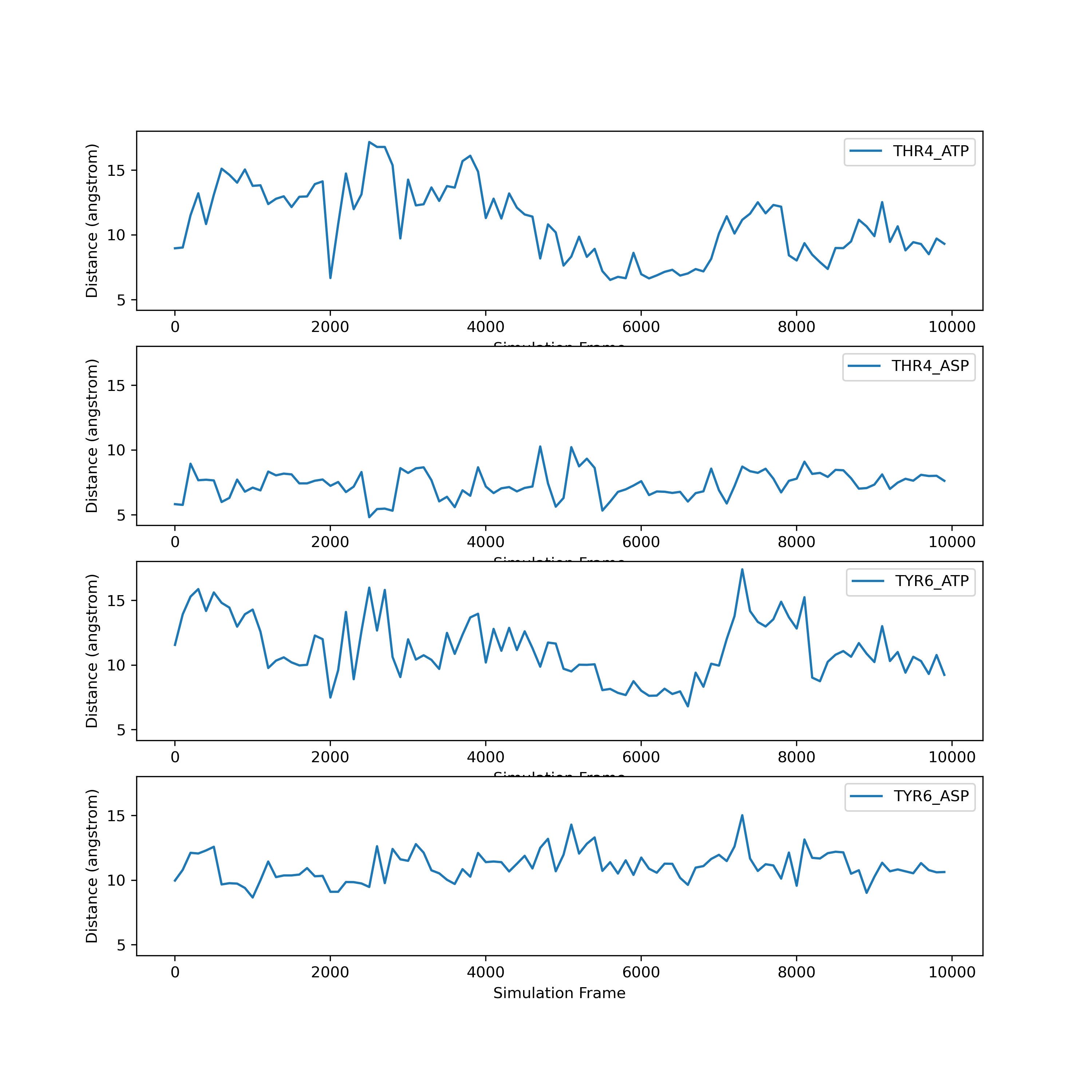
Matpotlib is highly customizable. What we’ve shown here is only the beginning of the types of plots you can make. If you would like to make more plots, we strongly recommend you check out the matplotlib tutorials online.
Key Points
The
matplotliblibrary is the most commonly used plotting library.You can import libraries with shorthand names.
You can save a figure with the
savefigcommand.Matplotlib is highly customizable. You can change the style of your plot, and there are many kinds of plots.
Writing Functions
Overview
Teaching: 25 min
Exercises: 15 minQuestions
How do I write include functions in my code?
Objectives
Define functions to perform one computational task.
Use functions within code and inside
forloops.Write functions that accept user inputs.
Assign default values for function inputs.
Why functions?
Most code is organized into blocks of code which perform a particular task. These code blocks are called functions. A commercial software package likely has hundreds of thousands or millions of functions. Functions break up our code into smaller, more easily understandable statements, and also allow our code to be more modular, meaning we can take pieces and reuse them. Functions also make your code easier to test, which we will see in a later lesson.
In general, each function should perform only one computational task.
Defining and running a function
In Python, the following syntax is used to declare a function:
def function_name(parameters):
** function body code **
return value_to_return
Functions are defined using the def keyword, followed by the name of the function. The function may have parameters which are passed to it, which are in parenthesis following the function name. A function can have no parameters as well. Most (though not all) functions return some type of information. It is important to note here that defining a function does not execute it.
Writing functions into our geometry analysis project
Let’s go back and consider a possible solution for the geometry analysis project.
import numpy
import os
file_location = os.path.join('data', 'water.xyz')
xyz_file = numpy.genfromtxt(fname=file_location, skip_header=2, dtype='unicode')
symbols = xyz_file[:, 0]
coordinates = xyz_file[:, 1:]
coordinates = coordinates.astype(numpy.float)
num_atoms = len(symbols)
for num1 in range(0, num_atoms):
for num2 in range(0, num_atoms):
if num1 < num2:
x_distance = coordinates[num1, 0] - coordinates[num2, 0]
y_distance = coordinates[num1, 1] - coordinates[num2, 1]
z_distance = coordinates[num1, 2] - coordinates[num2, 2]
bond_length_12 = numpy.sqrt(x_distance ** 2 + y_distance ** 2 + z_distance ** 2)
if bond_length_12 > 0 and bond_length_12 <= 1.5:
        print(F'{symbols[num1]} to {symbols[num2]} : {bond_length_12:.3f}')
To think about where we should write functions in this code, let’s think about parts we may want to use again or in other places. One of the first places we might think of is in the bond distance calculation. Perhaps we’d want to calculate a bond distance in some other script. We can reduce the likelihood of errors in our code by defining this in a function (so that if we wanted to change our bond calculation, we would only have to do it in one place.)
Let’s change this code so that we write a function to calculate the bond distance. As explained above, to define a function, you start with the word def and then give the name of the function. In parenthesis are in inputs of the function followed by a colon. The the statements the function is going to execute are indented on the next lines. For this function, we will return a value. The last line of a function shows the return value for the function, which we can use to store a variable with the output value. Let’s write a function to calculate the distance between atoms.
def calculate_distance(atom1_coord, atom2_coord):
x_distance = atom1_coord[0] - atom2_coord[0]
y_distance = atom1_coord[1] - atom2_coord[1]
z_distance = atom1_coord[2] - atom2_coord[2]
bond_length_12 = numpy.sqrt(x_distance ** 2 + y_distance ** 2 + z_distance ** 2)
return bond_length_12
Now we can change our for loop to just call the distance function we wrote above.
for num1 in range(0, num_atoms):
for num2 in range(0, num_atoms):
if num1 < num2:
bond_length_12 = calculate_distance(coordinates[num1], coordinates[num2])
if bond_length_12 > 0 and bond_length_12 <= 1.5:
print(F'{symbols[num1]} to {symbols[num2]} : {bond_length_12:.3f}')
Next, let’s write another function that checks to see if a particular bond distance represents a bond. This function will be called bond_check, and will return True if the bond distance is within certain bounds (At first we’ll set this to be between 0 and 1.5 angstroms).
def bond_check(atom_distance):
if atom_distance > 0 and atom_distance <= 1.5:
return True
else:
return False
This is great! Our function will currently return True if our bond distance is less than 1.5 angstrom.
Exercise
Modify the
bond_checkfunction to take a minimum length and a maximum length as user input.Answer
def bond_check(atom_distance, minimum_length, maximum_length): if atom_distance > minimum_length and atom_distance <= maximum_length: return True else: return False
Function Documentation
Recall from our work with tabular data that we were able to use help to see a help message on a function. As a reminder, we used it like this.
help(numpy.genfromtxt)
Help on function genfromtxt in module numpy.lib.npyio:
genfromtxt(fname, dtype=<class 'float'>, comments='#', delimiter=None, skip_header=0, skip_footer=0, converters=None, missing_values=None, filling_values=None, usecols=None, names=None, excludelist=None, deletechars=None, replace_space='_', autostrip=False, case_sensitive=True, defaultfmt='f%i', unpack=None, usemask=False, loose=True, invalid_raise=True, max_rows=None, encoding='bytes')
Load data from a text file, with missing values handled as specified.
Each line past the first `skip_header` lines is split at the `delimiter`
character, and characters following the `comments` character are discarded.
Let’s try the same thing on our function.
help(calculate_distance)
Help on function calculate_distance in module __main__:
calculate_distance(atom1_coord, atom2_coord)
There is no help for our function! That is because you haven’t written it yet. In Python, we can document our functions using something called docstrings. When you call help on something, it will display the docstring you have written. In fact, most Python libraries use docstrings and other automated tools to pull the docstrings out of the code to make online documentation. For example, see the documentation for the genfromtxt function online.
To add a docstring to our function, we simply add a block quote directly underneath the function definition. We do this in in the same way we type a string, except that we use three quotation marks to open and close the string instead of one.
def calculate_distance(atom1_coord, atom2_coord):
"""Calculate the distance between two three-dimensional points."""
x_distance = atom1_coord[0] - atom2_coord[0]
y_distance = atom1_coord[1] - atom2_coord[1]
z_distance = atom1_coord[2] - atom2_coord[2]
bond_length_12 = numpy.sqrt(x_distance**2+y_distance**2+z_distance**2)
return bond_length_12
We are using a very simple docstring in this example. However, there are many formats for docstrings. Now, you should see a message when you call help on this function.
help(calculate_distance)
Help on function calculate_distance in module __main__:
calculate_distance(atom1_coord, atom2_coord)
Calculate the distance between two three-dimensional points
If you use a well-known format, you can use software to extract the docstring and make a webpage with your documentation. Numpy-style docstrings are recommended. If you’re interested in learning more about developing python packages, there is a MolSSI course here: Python Package Development Best Practices Workshop.
Help vs Online Documentation
Many python libraries we have used such as numpy and matplotlib have extensive online documentation. It is a good idea to use online documentation if it is available. Typically, documentation for functions will be pulled from docstrings in the code, but additional information the code developers have provided will also be available through online documentation.
However, if you are offline or using a library without online documentation, you can check for documentation using the
helpfunction.
Remember, help for your code only exists if you write it! Every time you write a function, you should take some time to also write a docstring describing what the function does.
Function Default arguments
When there are parameters in a function definition, we can set these parameters to default values. This way, if the user does not input values, the default values can be used instead of the code just not working. For example, if we want the default values in bond check to be 0 and 1.5, we can change the function definition to the following:
def bond_check(atom_distance, minimum_length=0, maximum_length=1.5):
"""
Check if a distance is a bond based on a minimum and maximum bond length.
"""
if atom_distance > minimum_length and atom_distance <= maximum_length:
return True
else:
return False
Let’s try out the function now.
print(bond_check(1.5))
print(bond_check(1.6))
True
False
However, we can overwrite minimum_length or maximum_length.
print(bond_check(1.6, maximum_length=1.6))
Now that we have our bond_check function, we can use it in our for loop to only print the bond lengths that are really bonds.
num_atoms = len(symbols)
for num1 in range(0, num_atoms):
for num2 in range(0, num_atoms):
if num1 < num2:
bond_length_12 = calculate_distance(coordinates[num1], coordinates[num2])
if bond_check(bond_length_12) is True:
print(F'{symbols[num1]} to {symbols[num2]} : {bond_length_12:.3f}')
O to H1 : 0.969
O to H2 : 0.969
Exercise
We might also want to write a function that opens and processes our
xyzfile for us. Write a function called open_xyz which takes an xyz file as a parameter and returns the symbols and coordinates.Hint: You can return two values from a function by typing
return variable1, variable2.Answer
def open_xyz(filename): xyz_file = numpy.genfromtxt(fname=filename, skip_header=2, dtype='unicode') symbols = xyz_file[:, 0] coord = (xyz_file[:, 1:]) coord = coord.astype(numpy.float) return symbols, coord
We’ve now written three functions. Using these functions, our script to print bonded atoms now looks like this:
import numpy
import os
file_location = os.path.join('data', 'water.xyz')
symbols, coord = open_xyz(file_location)
num_atoms = len(symbols)
for num1 in range(0, num_atoms):
for num2 in range(0, num_atoms):
if num1 < num2:
bond_length_12 = calculate_distance(coord[num1], coord[num2])
if bond_check(bond_length_12) is True:
print(F'{symbols[num1]} to {symbols[num2]} : {bond_length_12:.3f}')
You can probably think of a further extension to use functions here. What if we wanted to print the bonds for another xyz file besides water? One option would be to copy and paste the two two for loops we’ve written. However, the smarter move is to put them in a function.
We could encapsulate the for loops into a function as well. Let’s do this, then perform the same analysis using both the water.xyz file and the benzene.xyz file.
First, we will define a new function print_bonds, which takes bond symbols and coordinates from an xyz file as an input.
def print_bonds(atom_symbols, atom_coordinates):
num_atoms = len(atom_symbols)
for num1 in range(0, num_atoms):
for num2 in range(0, num_atoms):
if num1 < num2:
bond_length_12 = calculate_distance(atom_coordinates[num1], atom_coordinates[num2])
if bond_check(bond_length_12) is True:
print(F'{atom_symbols[num1]} to {atom_symbols[num2]} : {bond_length_12:.3f}')
If you were to put all the functions we wrote into a single cell, it looks like this:
import numpy
import os
def calculate_distance(atom1_coord, atom2_coord):
"""
Calculate the distance between two three-dimensional points.
"""
x_distance = atom1_coord[0] - atom2_coord[0]
y_distance = atom1_coord[1] - atom2_coord[1]
z_distance = atom1_coord[2] - atom2_coord[2]
bond_length_12 = numpy.sqrt(x_distance ** 2 + y_distance ** 2 + z_distance ** 2)
return bond_length_12
def bond_check(atom_distance, minimum_length=0, maximum_length=1.5):
"""Check if a distance is a bond based on a minimum and maximum bond length"""
if atom_distance > minimum_length and atom_distance <= maximum_length:
return True
else:
return False
def open_xyz(filename):
"""
Open and read an xyz file. Returns tuple of symbols and coordinates.
"""
xyz_file = numpy.genfromtxt(fname=filename, skip_header=2, dtype='unicode')
symbols = xyz_file[:,0]
coord = (xyz_file[:,1:])
coord = coord.astype(numpy.float)
return symbols, coord
def print_bonds(atom_symbols, atom_coordinates):
"""
Prints atom symbols and bond length for a set of atoms.
"""
num_atoms = len(atom_symbols)
for num1 in range(0, num_atoms):
for num2 in range(0, num_atoms):
if num1 < num2:
bond_length_12 = calculate_distance(atom_coordinates[num1], atom_coordinates[num2])
if bond_check(bond_length_12) is True:
print(F'{atom_symbols[num1]} to {atom_symbols[num2]} : {bond_length_12:.3f}')
We can now open an arbitrary xyz file and print the bonded atoms. For example, to do this for water and benzene, we could execute a cell like this:
water_file_location = os.path.join('data', 'water.xyz')
water_symbols, water_coords = open_xyz(water_file_location)
benzene_file_location = os.path.join('data', 'benzene.xyz')
benzene_symbols, benzene_coords = open_xyz(benzene_file_location)
print(F'Printing bonds for water.')
print_bonds(water_symbols, water_coords)
print(F'Printing bonds for benzene.')
print_bonds(benzene_symbols, benzene_coords)
Printing bonds for water.
O to H1 : 0.969
O to H2 : 0.969
Printing bonds for benzene.
C to H : 1.088
C to C : 1.403
C to C : 1.403
C to H : 1.088
C to C : 1.403
C to H : 1.088
C to C : 1.403
C to H : 1.088
C to C : 1.403
C to H : 1.088
C to C : 1.403
C to H : 1.088
Volume function
In earlier lessons, we extracted the cell lengths of multiple cif files using
glob. With the a, b, and c cell lengths, we can calculate the volume of the cell, V = abc. Write a function that takes the three cell lengths and returns the volume. Add it to your previous code and output a new file, “orthorhombic_cell_data_vol.txt” which includes all the previous information and a new column for cell volume.Solution
# Here's one possible function to calculate the volume of an orthorhombic cell
def orthorhombic_volume(cell_a, cell_b, cell_c):
    """Calculate the volume of an orthorhombic cell, V = abc"""

    volume = cell_a * cell_b * cell_c
    return volume
.
Extension
Looking at your cif file processing code, what other parts could be made into functions?
Solution
# We can write a function to get the filename (though there are already functions in the "os" library to  do this
def get_filename(filename):
    """Given a filename, including a path, return just the filename without extension"""
    file_name = os.path.basename(filename)
    split_filename = file_name.split('.')
    molecule_file_name = split_filename[0]
    return molecule_file_name

# We can also write a function to return the three cell dimensions. Here's one possible function
def get_cell_dimensions(data):
    """Return a tuple of the three cell dimensions from a read in cif file"""
    #In case something is not read in correctly, set all cell values to zero
    cell_a = 0
    cell_b = 0
    cell_c = 0
    for line in data:
        if '_cell_length_a' in line:
            cell_dimension_a_line = line
            words = cell_dimension_a_line.split()
            cell_a = float(words[1])
        elif '_cell_length_b' in line:
            cell_dimension_b_line = line
            words = cell_dimension_b_line.split()
            cell_b = float(words[1])
        elif '_cell_length_c' in line:
            cell_dimension_c_line = line
            words = cell_dimension_c_line.split()
            cell_c = float(words[1])

    return (cell_a, cell_b, cell_c)

# And a function to extract the molecule systematic name
def get_molecule_systematic_name(data):
   """Returns the systematic name of the molecule. Returns None if not found."""
   molecule_name = None
   for linenum, line in enumerate(data):
       if '_chemical_name_systematic' in line:
           name_line = linenum + 2
           molecule_name = data[name_line].rstrip('\n') #We use rstrip() to remove the newline character
   return molecule_name

# Using the functions we've defined, our original code now becomes quite short:
file_location = os.path.join('structures', 'orthorhombic', '*.cif')#*
import glob
filenames = glob.glob(file_location)
#print(filenames)

#open output file for writing
datafile = open('orthorhombic_cell_data_vol.txt','w+')
datafile.write(F'Molecule Filename \t Molecule Name \t cell_a \t cell_b \t cell_c\n')
for f in filenames:
   # Get the file name of the individual file
   molecule_file_name = get_filename(f)

   # Read the data
   ciffile = open(f,'r')
   data = ciffile.readlines()
   ciffile.close()
   #print(data)

   molecule_systematic_name = get_molecule_systematic_name(data)
   (cell_a, cell_b, cell_c) = get_cell_dimensions(data)

   volume = orthorhombic_volume(cell_a, cell_b, cell_c)

   #Now write to the file
   datafile.write(F'{molecule_file_name} \t {molecule_systematic_name} \t {cell_a} \t {cell_b} \t {cell_c}\t {volume}\n')

datafile.close()
Key Points
Functions make your code easier to read, more reuseable, more portable, and easier to test.
If a function returns True or False, you can use it in an
ifstatement as a condition.
The Atomic Simulation Environment: Python for Chemistry
Overview
Teaching: 25 min
Exercises: 15 minQuestions
How can I use python to manipulate molecules ?
Objectives
Read and view molecules from different format files
Manipulate molecules and write to new files
Set up a calculator and use it for a molecule.
Atomic Simulation Environment
The Atomic Simulation Environment (ASE): https://wiki.fysik.dtu.dk/ase/ is a tremendously powerful set of tools and Python modules for setting up, manipulating, running, visualizing and analyzing atomistic simulations.
Atoms in the ASE
In episode 1, you wrote python dictionaries to describe the three carbon atoms in acetone. You might have come up with something like this:
atom ={
"atomic number": 6
"atomic symbol": "C"
"isotope": 12
"charge": 0
"position": [0.0, 0.0, 0.0]
}
ASE provides an Atom object to store and manipulate atoms in chemical simulations. The Atom object is a python class defined here. Compare the data types of the Atom parameters with your dictionary.
Just like floats or strings can be put into lists, ASE also defines a collection of atoms. The Atoms object is defined here
Let’s make up a simple molecule (a.k.a. Atoms object) and view it:
from ase import Atoms
d = 1.1
co = Atoms('CO', positions=[(0, 0, 0), (0, 0, d)])
from ase.visualize import view
view(co, viewer='x3d')
This will bring up a viewer in you your Jupyter notebook, you can rotate the molecule using the mouse.
Let’s read in a more complex molecule: From the NOW page, the file caffeine.xyz should have been downloaded with all the files for this course:
from ase.io import read, write
caffeine = read("caffeine.xyz")
view(caffeine, viewer='x3d')
The ASE has internally defined many methods to read (and to write) common chemical formats. When you use the read function that you imported from ase.io, it determed the filetype from its extension (xyz) and uses the appropriate function to read the file and return an Atoms object.
You can also read and view the Cu(OH)2 crystal you used in an earlier episode:
cuoh = read("CuOH.cif")
view(cuoh, viewer='x3d')
Manipulating molecules
As you saw above, when you created a CO molecule, ASE allows you to manipulate the positions of atoms directly. There are many methods that can be used on Atoms objects, they are all listed, with examples here. Let’s look at two water molecules:
two_waters = read("2_h2o.xyz")
view(two_waters, viewer='x3d')
You might want to look at the molecule using a full molecular viewer (e.g. the free, open-source IQMol) to see how the two water molecules are arranged, but we can also do this in python:
print(two_waters.symbols)
print(two_waters.positions)
OH2OH2
[[ 0.        0.        0.      ]
 [-0.223085 -0.94174   0.      ]
 [ 0.976851  0.        0.      ]
 [ 2.895318  0.        0.      ]
 [ 3.095395  0.561093  0.765582]
 [ 3.095395  0.561093 -0.765582]]
So the first atom is an oxygen atom at position [0.0, 0.0, 0.0], the next two atoms are hydrogen atoms, the fourth atom (index = 3 in python!) is an oxygen atom with coordinates of [2.895318, 0.0, 0.0]. We could print this information more clearly using a loop:
for atom in two_waters:
    print(atom.symbol, atom.position)
O [0. 0. 0.]
H [-0.223085 -0.94174   0.      ]
H [0.976851 0.       0.      ]
O [2.895318 0.       0.      ]
H [3.095395 0.561093 0.765582]
H [ 3.095395  0.561093 -0.765582]
To move the second water molecule away from the first, we can translate the last three atoms. If we decide to translate the molecule along the x-axis, we can simply increase the x-coordinate of the second molecule (half of the Atoms object):
translation = 2.0
two_waters.positions[3:] += ([translation, 0.0, 0.0])
for atom in two_waters:
    print(atom.symbol, atom.position)
view(two_waters, viewer='x3d')
O [0. 0. 0.]
H [-0.223085 -0.94174   0.      ]
H [0.976851 0.       0.      ]
O [6.895318 0.       0.      ]
H [7.095395 0.561093 0.765582]
H [ 7.095395  0.561093 -0.765582]
The molecule shown in the viewer looks different from before, but it is hard to tell from the viewer that we’ve changed the molecule, though we can see from the printed coordinates that we have indeed changed them. Let’s write out the new molecule, so we can view it in IQmol:
new_waters = '2_h2o_new.xyz'
write(new_waters, two_waters)
This command won’t appear to do anything, but you should have a new file called 2_h2o_new.xyz in your directory. Open it, either as a text file, or in IQmol and compare it to the original file that you read in.
We can also determine (get_) and change (set_) angles and dihedral angles. Dihedral angles are also called torsions, if you’ve not heard of a dihedral angle before, a good explanation is here.
two_waters = read("2_h2o.xyz")
original_dihedral = two_waters.get_dihedral(1,0,3,5)
print(original_dihedral)
two_waters.set_dihedral(1,0,3,5,240,[0,0,0,1,1,1])
view(two_waters, viewer='x3d')
The output will show the dihedral angle to far too many decimal places (1 is enough) and then will show the molecule viewer, where you verify that the second water molecule is now in a different orientation compared to the molecule you read in:
126.23758921152063
If you’d like to make absolutely certain that you’ve changed the molecule, write it out to a new file and view it in IQmol.
Setting up a calculator
ASE can also act as an interface to several computational chemistry programs that can optimise the geometry of the molecule, determine the vibrational (IR) spectrum of the molecule and simulate the molecule over time by running molecular dynamics, amongst many other things. A calculator in ASE is an interface to one of these programs that sends the Atoms object to the program and (after some time, which may be less than a second, or even up to several hours), receives some information back from the program. The most common piece of information for a calculator to return, is a potential energy and we’ll focus on that in this episode. To use an ASE calculator, we first have to import it, set it up and attach it to our Atoms object. For this example, we’ll use a very straightforward calculator, designed especially for water, called TIP4P.
#Import
from ase.calculators.tip4p import TIP4P
#Setup calculator, TIP4P doesn't need any options, so we just need to define it
calc = TIP4P()
#Read in molecule to a new Atoms object
two_waters = read("2_h2o.xyz")
#Attach the calculator to our Atoms object
two_waters.set_calculator(calc)
print(two_waters.get_potential_energy())
-0.266677737333415
The output is the energy of the two water molecules in electron Volts (eV).
Exercise
Determine the optimal distance and the binding energy of the two water molecules. Change the distance between the molecules between [-0.5:1.5] Angstrom in 0.01 Angstrom increments.
Answer
from ase.calculators.tip4p import TIP4P
calc = TIP4P()
# Set up empty lists for energies and distances
energies = []
distances = []
# We're asked to determine the distance at the minimum energy, so setup variables for minimum energy and distance
minimum_energy = 0.0
optimum_distance = 0.0
# Now read the molecule
two_waters = read("2_h2o.xyz")
# Find out the initial distance between the two waters
initial_H_bond_length = two_waters.get_distance(2,3)
print(F'Initial Hydrogen bond distance read in from file = {initial_H_bond_length} Angstrom')
# Now we need a loop to change the distance between the two water molecules and calculate the energy each time
for distance in range(-50,150):
    molecule = two_waters.copy() #Use a copy of the molecule to make sure we get exactly the distance we want
    molecule.set_calculator(calc)
    molecule.positions[3:] += ([distance * 0.01, 0.0, 0.0])
    distances.append(initial_H_bond_length + distance * 0.01)
    energies.append(molecule.get_potential_energy())
    #Now check if our energy is less than our current minimum energy:
    if molecule.get_potential_energy() < minimum_energy:
        minimum_energy = molecule.get_potential_energy()
        optimum_distance = initial_H_bond_length + distance * 0.01

print(F'Optimal Hydrogen bond distance (TIP4P) = {optimum_distance} Angstrom')
print(F'Binding energy at that distance = {minimum_energy} eV' )
ax = plt.gca()
ax.plot(distances, energies)
ax.set_xlabel('Distance [Å]')
ax.set_ylabel('Total energy [eV]')
plt.show()
Key Points
The ASE can be used to read, write and manipulate most common chemical formats.
Calculators in ASE interface with a variety of compuational chemistry programs.
Because the ASE is in python, we can use it to do a chemical calculation and use other python modules (e.g. numpy, matplotlib) to use the results of calculations.